| Home | Papers | Reports | Projects | Code Fragments | Dissertations | Presentations | Posters | Proposals | Lectures given | Course notes |
|
|
Antenna Finding and Interpolation/Extrapolation of Signal StrengthWerner Van Belle1* - werner@yellowcouch.org, werner.van.belle@gmail.com Abstract : This article investigates the possibility to determine the position of a WiFi antenna by sampling the environment using a standard wireless card. The method is based on a search algorithm (simulated annealing) in a renormalized antenna model. The article further documents a sample acquisition phase in which a static wireless card measured the local environment. This might allow the integration of various oscillatory phenomena into the model.
Keywords:
antenna finding, transmitter finding, WiFi, wireless networks |
Contents
- List of Figures
- 1 Introduction
- 2 Local Interpolation using Thin Plate Splines
- 3 Transmitter Finding
- 4 Sampling WiFi Signals
- 5 Conclusion
- Bibliography
1 Introduction
|
This article investigates the possibility to determine the position of a WiFi base station using irregular sampling. Based on various sample points we try to interpolate the expected signal strength. Sample points are acquired using 'samplers', which are mobile transceivers. The position of a sampler is however not under our control. Each sampler records position, time and signal strength of all available base stations. The signal strengths at the same position can vary greatly (mist, outliers). We want to integrate those irregular sampled points into a coherent signal map, which is half symbolic and half numerical. The symbolic part indicates the base station identifier, the numerical part reports on the strength of that specific base station identifier.
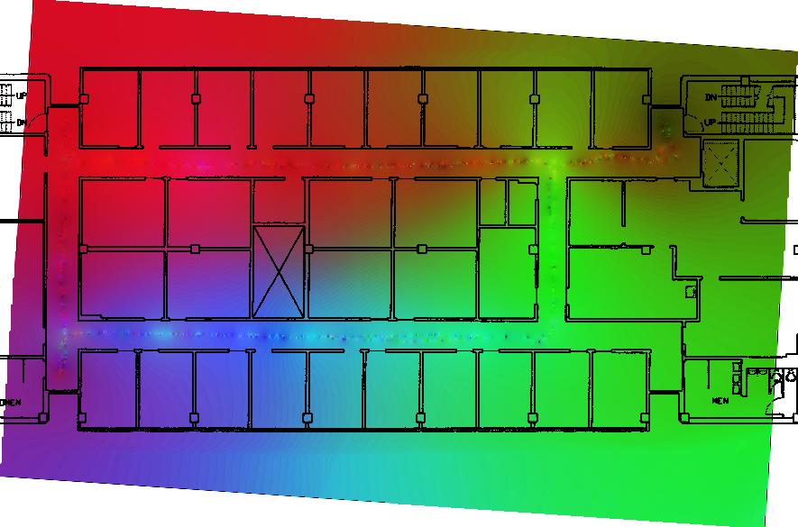
The general goal of such a map is to be able to predict the signal strength of yet unknown areas. Figure 1 gives an example of a WiFi signal strength map with 3 base stations in a building. The topic on signal strength interpolation itself has received some attention due to the possibility to determine the position based on the signal strengths of various antennas [3].
The first section of the article handles the problem of interpolating signal strength, or differently stated: given a small number of samples, that might contain errors both in position and signal strength, how can we assess the signal strength of nearby position. This problem also includes the problem of local variations and blind spots in antenna coverage due to buildings, land mass, reflections and so on. The second section investigates the possibility to find the position of an transmitter using simulated annealing on a renormalized antenna model. This is typically achieve by integrating expected physics (inverse square) into a framework of sample points. Up-sampling in general is done by means of expanding the signal and then getting the signal through a low-pass filter of appropriate design. The third part focuses on some practical experiments. This will give us more insight in the nature of WiFi communication. This includes understanding the variance one might expect, whether the time of day and date are related to signal strength, how cross correlations between wireless stations can be handled and whether there are signal strength oscillations that we need to take into account.
2 Local Interpolation using Thin Plate Splines
In this part we investigate the problem of extrapolating and interpolating signal strength of one WiFi base station (isotropic transmitter) based on a number of sample points that might have errors both in the measured signal strength as well as the current position.
2.1 Thin Plate Splines
|
The interpolation between various 2 dimensional points appears similar
to the interpolation problem of 3 dimensional points. To understand
this one must realize that the signal strength can be set out as the
![]() -axis while the coordinate
-axis while the coordinate ![]() and
and ![]() represent the geographical
position. Splines are well defined in 2 and 3 dimensions and are based
on preserving the smoothness of a curve as good as possible. Splines
can have either a fixed (static first order differential) or non-fixed
end (non-static first order differential). If they have a fixed end
then the slope in those points must be zero in all directions. Which
brings us to the interesting question: how well developed are thin
plate splines to represent sampled magnetic fields without knowing
the actual source of the transmission. Research regarding splines
can be found in [5, 4, 6, 7, 8, 9, 10].
Extensions exist that are better suited to handle discontinuities
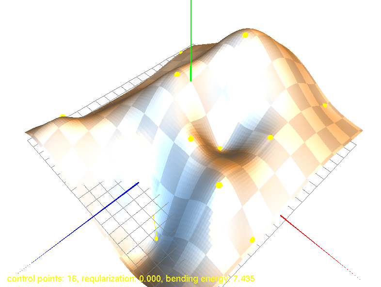
(such as walls) [11, 12]. Figure 2
shows how such splines look like. We tested a number of simple problems
to see how TPS performs.
represent the geographical
position. Splines are well defined in 2 and 3 dimensions and are based
on preserving the smoothness of a curve as good as possible. Splines
can have either a fixed (static first order differential) or non-fixed
end (non-static first order differential). If they have a fixed end
then the slope in those points must be zero in all directions. Which
brings us to the interesting question: how well developed are thin
plate splines to represent sampled magnetic fields without knowing
the actual source of the transmission. Research regarding splines
can be found in [5, 4, 6, 7, 8, 9, 10].
Extensions exist that are better suited to handle discontinuities
(such as walls) [11, 12]. Figure 2
shows how such splines look like. We tested a number of simple problems
to see how TPS performs.
2.2 Sample Scenarios
In what follows we tested the interpolation/extrapolation capabilities based on a number of simulated sample points. These were taken from a map of calculated transmission at specific points.
- The first scenario simulates a sampler that goes linearly through a coverage area and irregularly samples the signal strength. The question now how good TPS will be able to predict other points ?
- The second scenario samples two samplers walking orthogonal to each other.
- This scenario samples a number of points at random around the antenna
- This scenario samples a number of points before the antenna. Will our predictor be able to extrapolate the other side of the antenna ?
2.3 TPS Interpolation/Extrapolation
|
Based on these sample points we interpolated a new signal strength map (middle column of figure 3), after which we measured the error between the proper map and the interpolated map (third column in figure 3). Our overall assessment is that the prediction is locally correct, but that it is unable to properly extrapolate, nor interpolate properly near the exponentially increasing antenna.
- In case a sampler always follows the same route, then an estimation will be very accurate for that zone.
- If many different points are uniformly sampled then the estimate is quite correct, except for positions close to the base station there we find the the TPS estimation always underestimates the slope.
- If only one side of a base station is sampled then the other side cannot be extrapolated properly.
- Since the TPS formalism will fit the spline through every point we end up with problems when measurement errors occur. E.g: one sampler measuring no signal (mist or so, or bad hardware). Then the spline interpolation will go through it entirely.
- This model is accurate for local estimates but it fails to take into account the quickly changing center and the symmetry around the center.
3 Transmitter Finding
3.1 The Transmission Model
This section concerns itself with the problem of estimating the
position
of the antenna. This will make it possible to model the energy
landscape
based on a very simple formula. To find the transmitter-center, we
assume that we have an exponential decaying signal such as
![]() .
In practice electromagnetic waves decay based on the permeability
of the ether (
.
In practice electromagnetic waves decay based on the permeability
of the ether (![]() )
and the strength of the original signal.
It is often measured in decibels, related to some unit power (e.g.
dBm). We can model the signal-strength as
)
and the strength of the original signal.
It is often measured in decibels, related to some unit power (e.g.
dBm). We can model the signal-strength as
in which ![]() is a constant
based on the current weather conditions
is a constant
based on the current weather conditions
![]() .
. ![]() is the distance to the transmitter. To
determine
the transmitter position
is the distance to the transmitter. To
determine
the transmitter position ![]() based on a
set
of sample points
based on a
set
of sample points ![]() ,
, ![]() and
and
![]() we need to solve the following set of
equations:
we need to solve the following set of
equations:
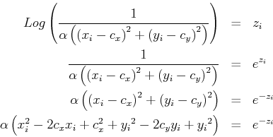
3.2 Direct use
of expected signal strength
Such a system of equations is difficult to solve using Gauss-Jordan
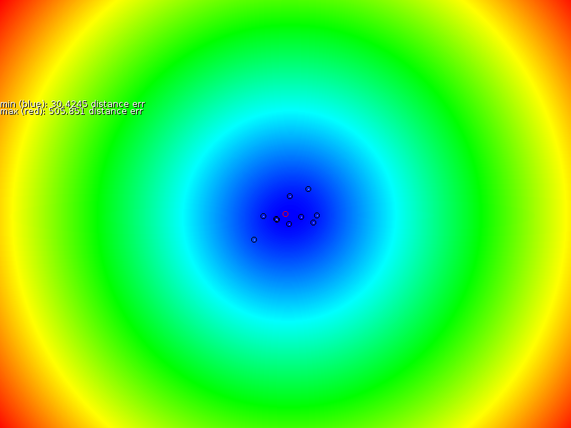
and standard linear equations. We first resorted to a brute force
numerical algorithm that for every pixel in the area determined how
big the error between the estimated signal strength and the measured
signal strength was. With the proper scaling factor ![]() the
results were determined as follows.
the
results were determined as follows.
|

Calculating ![]() for one
position requires
for one
position requires ![]() operations (
operations (![]() being the
number of samples). So, for the entire
map we have
being the
number of samples). So, for the entire
map we have ![]() calculations.
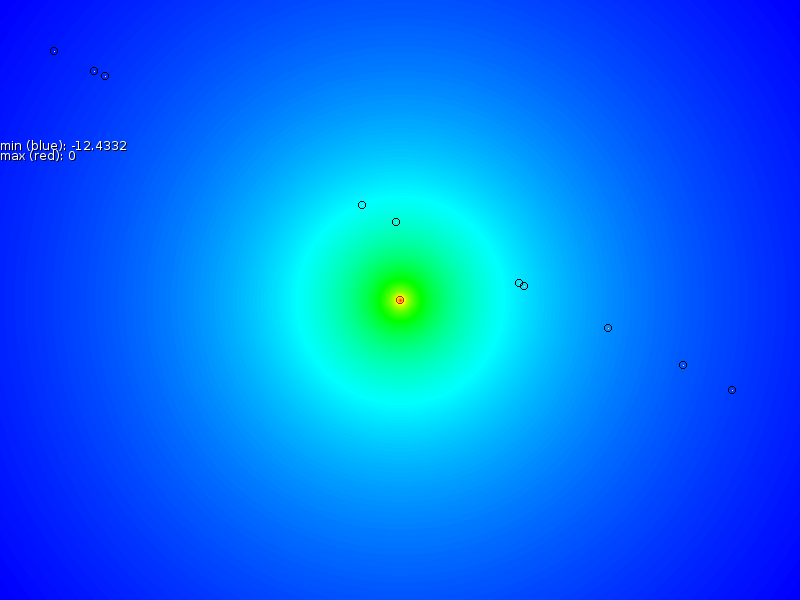
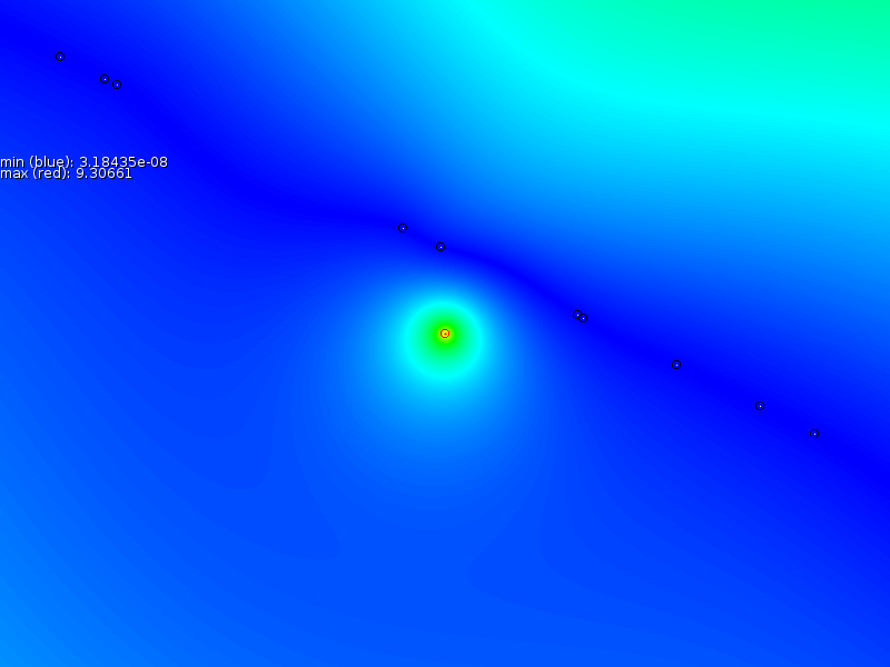
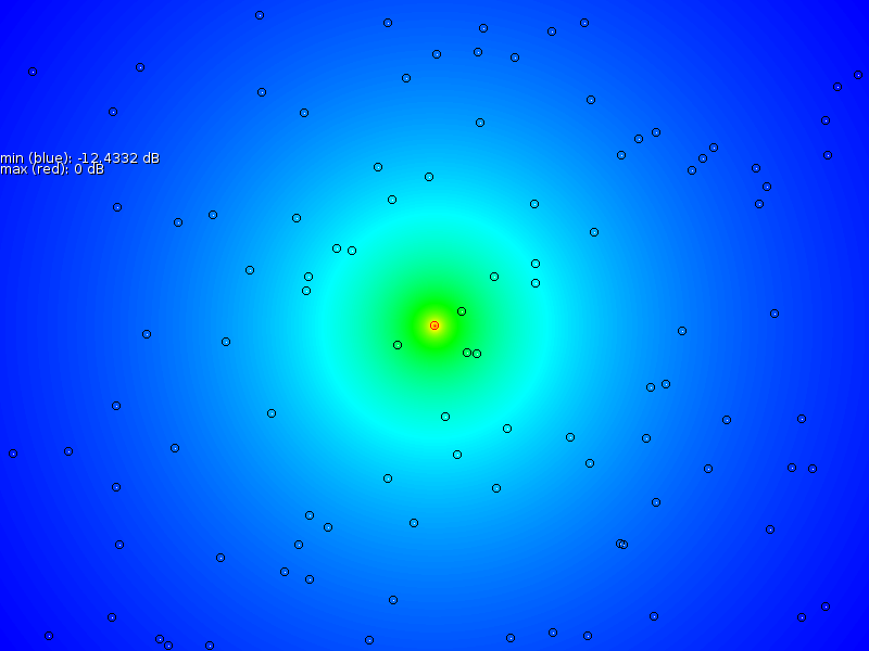
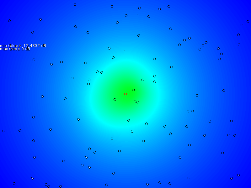
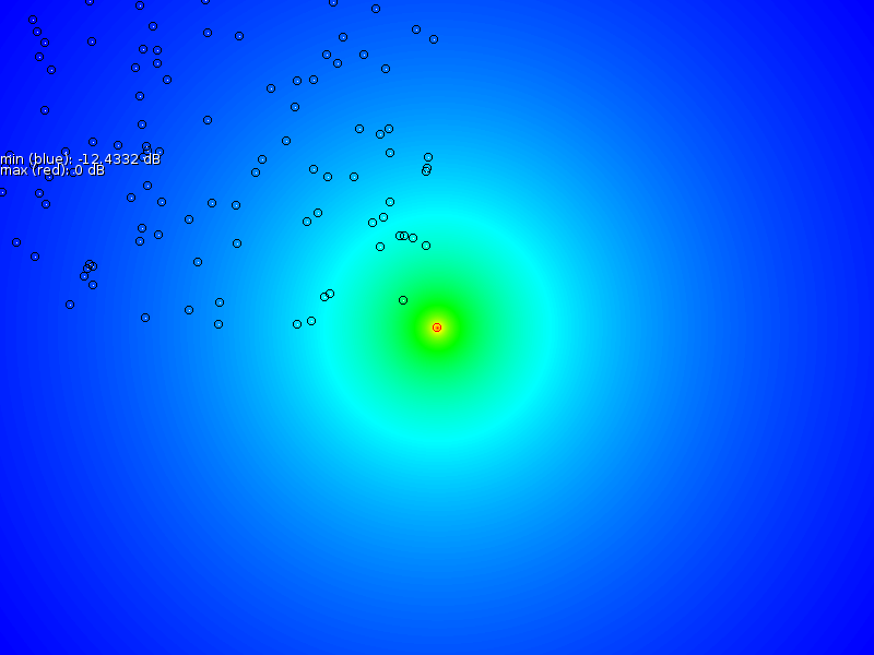
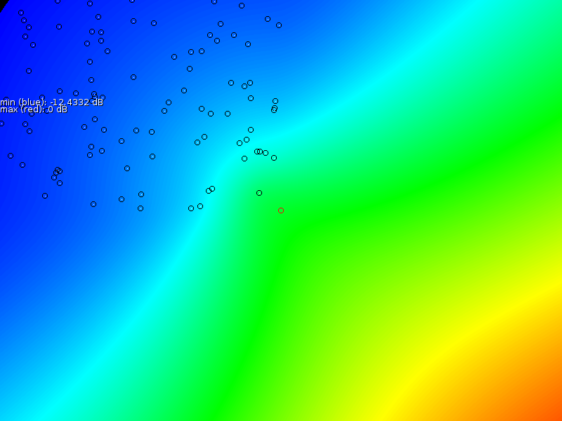
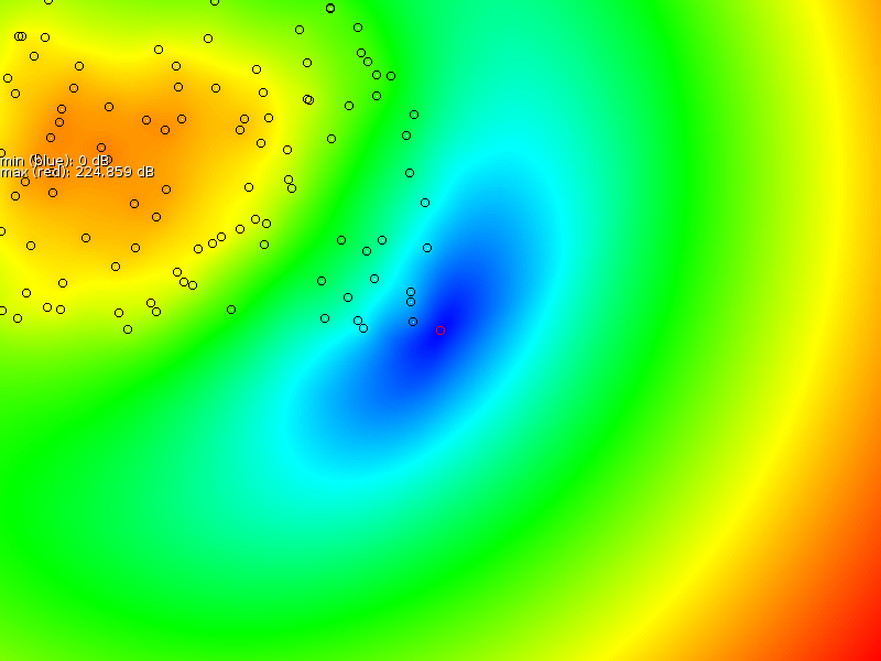
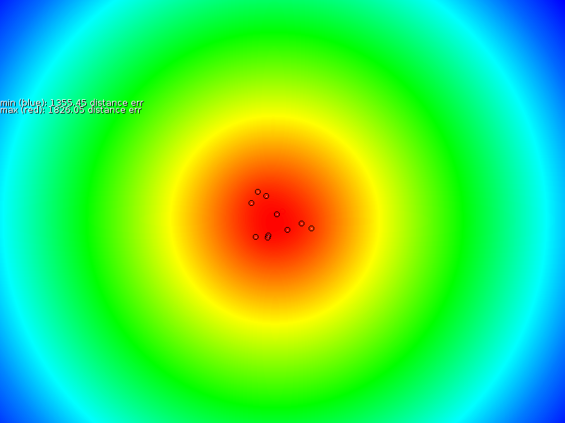
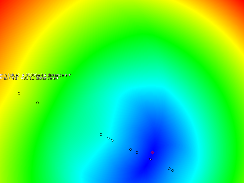
Figure 4 shows the result of such
a map.
Blue are the areas where the mismatch would be minimal if the
transmitter
was located at that position. Red are areas that do not match at all.
By experimenting with values of
calculations.
Figure 4 shows the result of such
a map.
Blue are the areas where the mismatch would be minimal if the
transmitter
was located at that position. Red are areas that do not match at all.
By experimenting with values of ![]() it became clear that the
found center would actually shift if
it became clear that the
found center would actually shift if ![]() was chosen badly. As
such, the presented method is useful for educative purposes it will
not live up to the test in real environments, since there we will
need to estimate
was chosen badly. As
such, the presented method is useful for educative purposes it will
not live up to the test in real environments, since there we will
need to estimate ![]() as well.
as well.
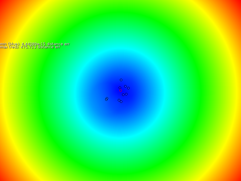
To resolve this
problem we investigated a
more suitable algorithm
for our purpose: simulated annealing combined with a simplex
minimization
algorithm [VF02a]. By
using 2 we tried
to find ![]() ,
, ![]() and
and ![]() automatically. Here
it turned out
that there are many local minimal solutions outside the box.
Specifically
when
automatically. Here
it turned out
that there are many local minimal solutions outside the box.
Specifically
when ![]() is very
large, or when
is very
large, or when ![]() is far outside
the sampling area, then we find that
is far outside
the sampling area, then we find that ![]() mainly measures
mainly measures ![]() ,
which itself is a much smaller error than position nearby the sampling
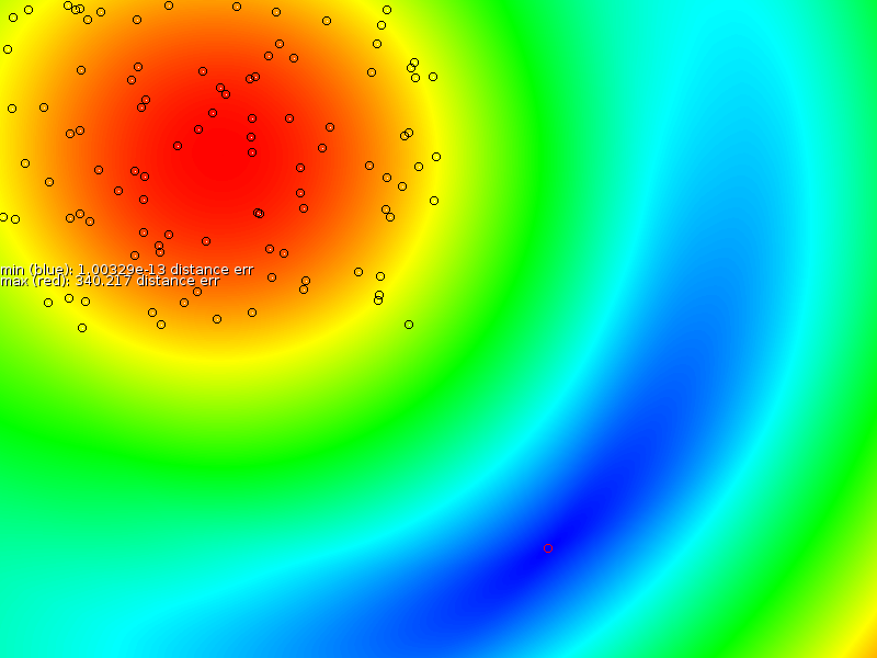
area. This explains why the simulated annealing procedures combined
with equation 2 can suddenly fall
outside
the area
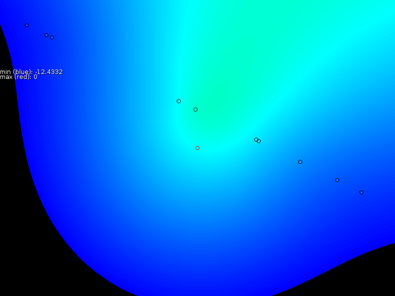
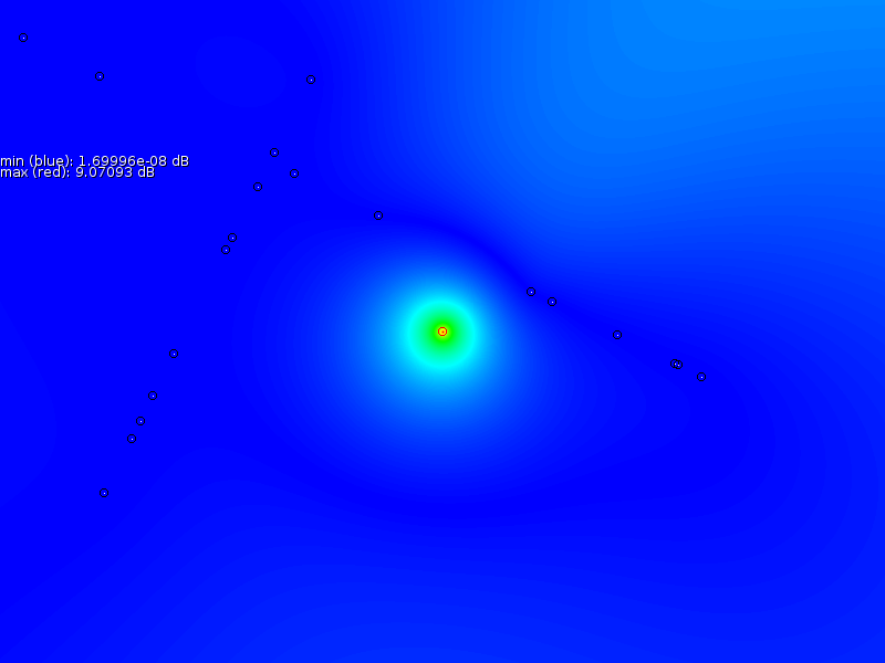
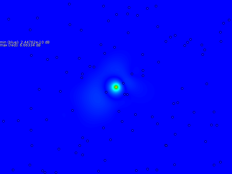
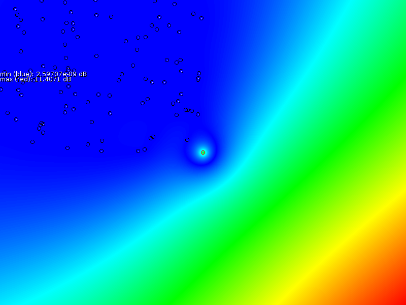
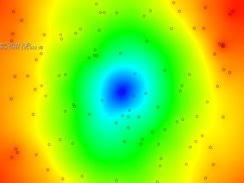
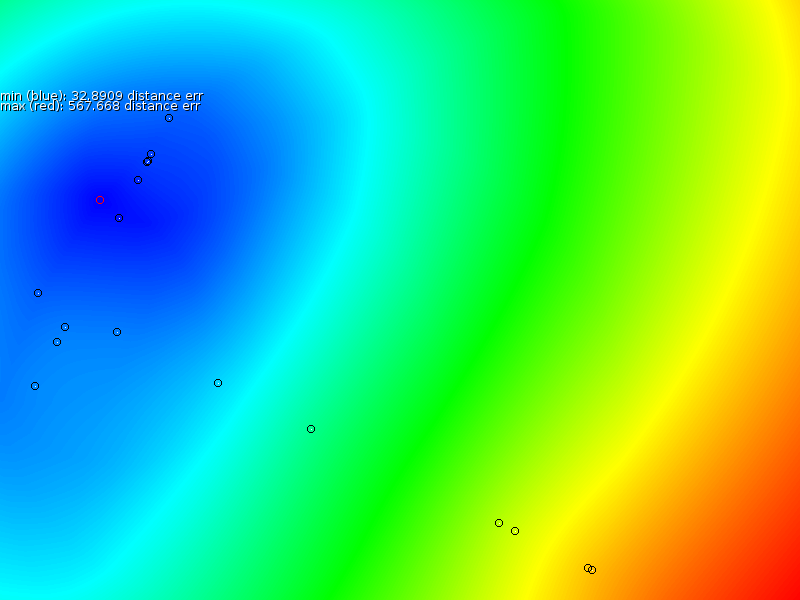
and not enter it again. To illustrate this point further, we created
a much larger map that illustrates how the error function reacts on
large distances or large
,
which itself is a much smaller error than position nearby the sampling
area. This explains why the simulated annealing procedures combined
with equation 2 can suddenly fall
outside
the area
and not enter it again. To illustrate this point further, we created
a much larger map that illustrates how the error function reacts on
large distances or large ![]() values
(Fig. 5).
values
(Fig. 5).
3.3 Renormalization
|


From the experiment in section directUse, we find that the
error function ![]() might not be
a proper choice. Therefore
we went back to the basic questions: a) what do we want to minimize
and b) can we renormalize
might not be
a proper choice. Therefore
we went back to the basic questions: a) what do we want to minimize
and b) can we renormalize ![]() to avoid low signals at improbably
positions ? The answer to a is: the error in the position estimation.
However, since
to avoid low signals at improbably
positions ? The answer to a is: the error in the position estimation.
However, since ![]() goes through
an inverse function and a logarithm
we have a very inconsistent energy landscape in which to find the
minimal mismatch position.
goes through
an inverse function and a logarithm
we have a very inconsistent energy landscape in which to find the
minimal mismatch position.
As
such we tried to get rid of the
inverse and log functions by,
instead
of using the dB scale, using a distance scale as input in the error
function. Instead of measuring the signal strength in dBm we convert
it to its actual distance by taking the inverse and sqrt-ing it. So
if ![]() is the measurement at a
specific position, of which the distance
to the antenna is not know then we can simply take
is the measurement at a
specific position, of which the distance
to the antenna is not know then we can simply take
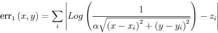
![]() as a linear
correlate to the distance function. So , to realize b),
we must replace
as a linear
correlate to the distance function. So , to realize b),
we must replace ![]() with
with
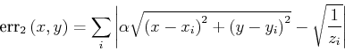
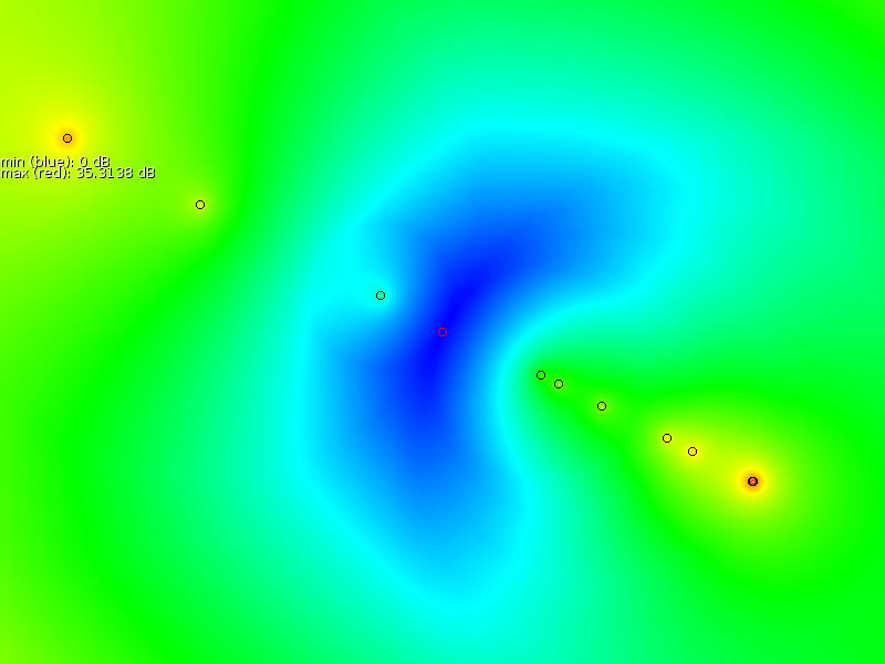
|
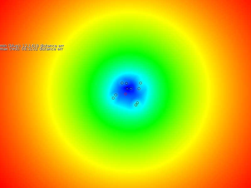
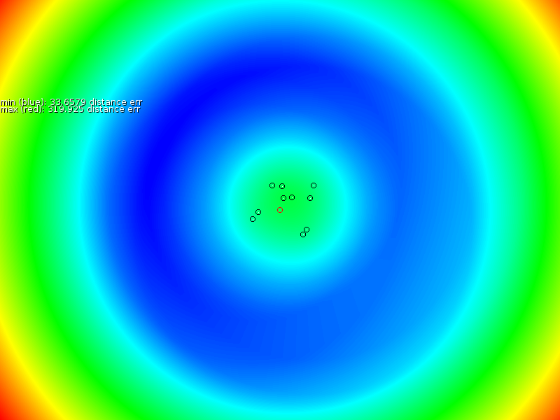
This error function will become larger for all values far away from
the sampling area as well as it will become large for positions where
we barely find a signal. What one can do know is simply walk this
novel reorganized landscape and find the minimum. A quick test on
this method shows that it is a very good solution to the presented
problem. It makes it possible to estimate ![]() ,
, ![]() and
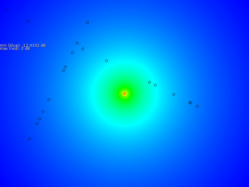
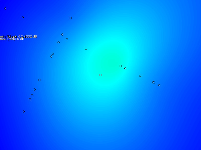
and ![]() fairly accurate. Figure 6 shows the
various
outputs. Furthermore since the measurement scale becomes linear, it
also becomes a good set of input functions for thin plate splines.
fairly accurate. Figure 6 shows the
various
outputs. Furthermore since the measurement scale becomes linear, it
also becomes a good set of input functions for thin plate splines.
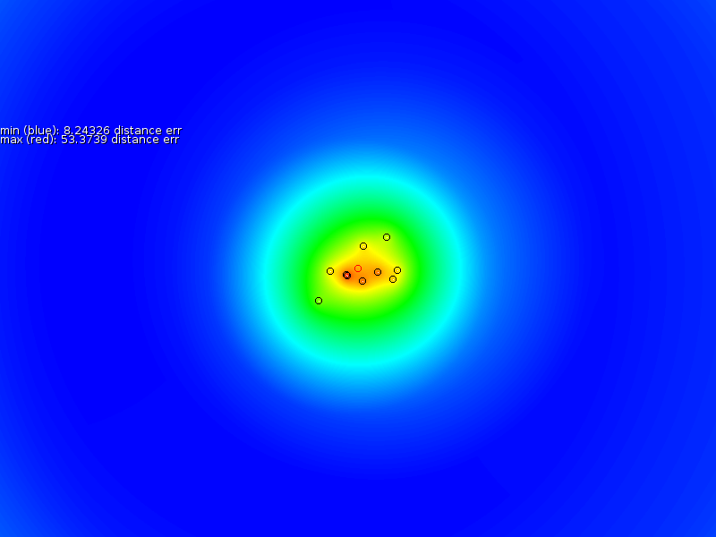
3.4 Error sensitivity
Further tests on equation 3 revealed that is is not sensitive to outliers and that jitter slightly influences the outcome. It will actually be able to estimate the transmitter position better than the underlying accuracy of the position measurement. However, in a practical setting these are not expected to form a problem.
4 Sampling WiFi Signals
The description in previous part is important from a modeling point of view. Now that the theoretical side has been approached, we need to conduct a number of test to get a 'feeling' for WiFi zones. This include verifying whether there is a relation between the time of day/day of week/day of month and signal availability as well as measuring some upper/lower-bounds on the signal strength variance and signal quality variance.
4.1 Test Procedure & Units
|
|
As a small experiment we have been sampling our direct environment from a static WiFi card. The information was taken with iwlist scan and parsed using various scripts. The reports include both signal strength (expressed in dBm) and signal quality (expressed in %). The unit of the signal strength is measured by the WiFi card as dBm, which does not stand for dB meter but rather dB miliWatt. Zero dBm equals one milliwatt. A 3 dB increase represents roughly doubling the power, which means that 3 dBm equals roughly 2 mW. For a 3 dB decrease, the power is reduced by about one half, making 3 dBm equal to about 0.5 milliwatt [13]. The formula to obtain dBm from power is given as
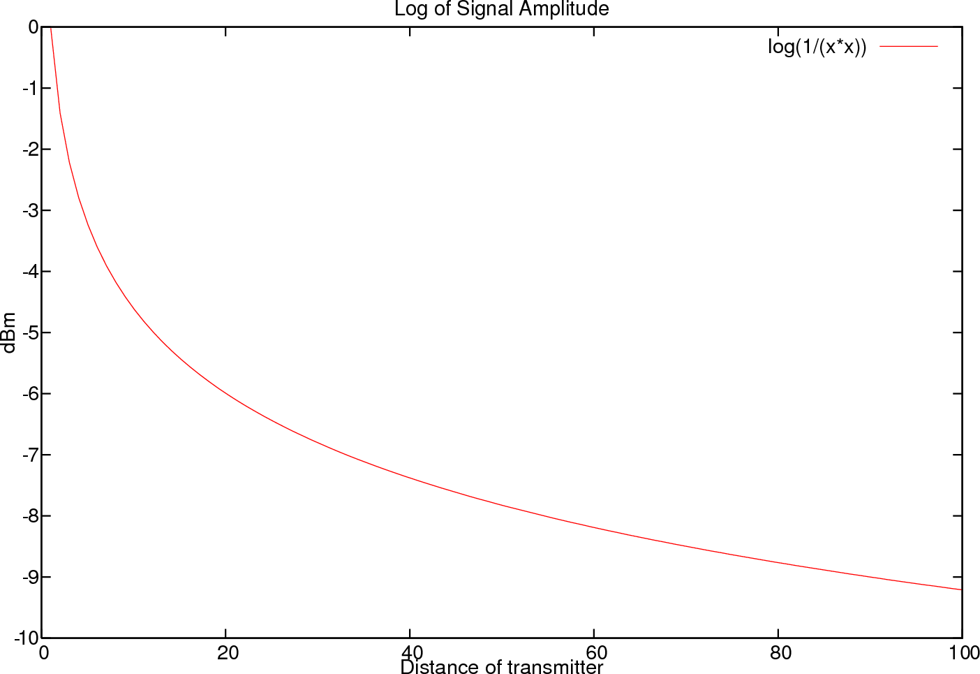
If we take into account the distance and define ![]() as
as ![]() ,
then we can directly relate dBm to our model (eq. eq:w)
,
then we can directly relate dBm to our model (eq. eq:w)
Figure 7 illustrates how such a decaying signal will look like, if we assume that this model is correct.
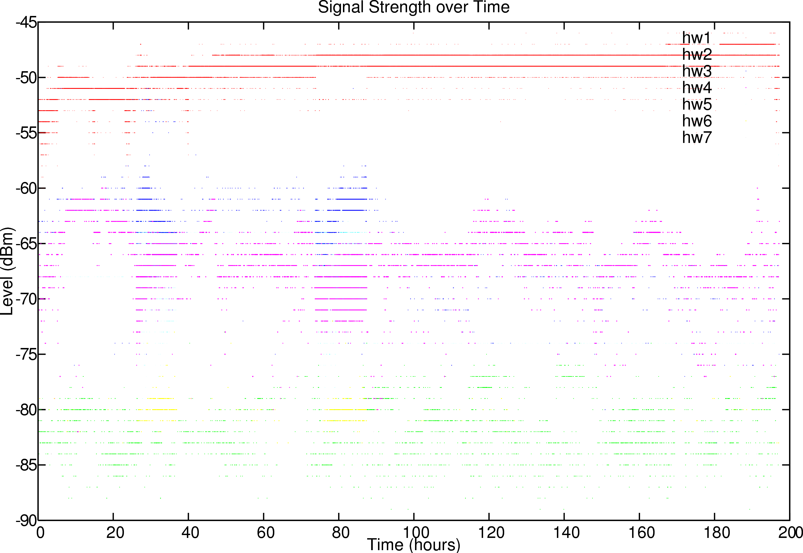
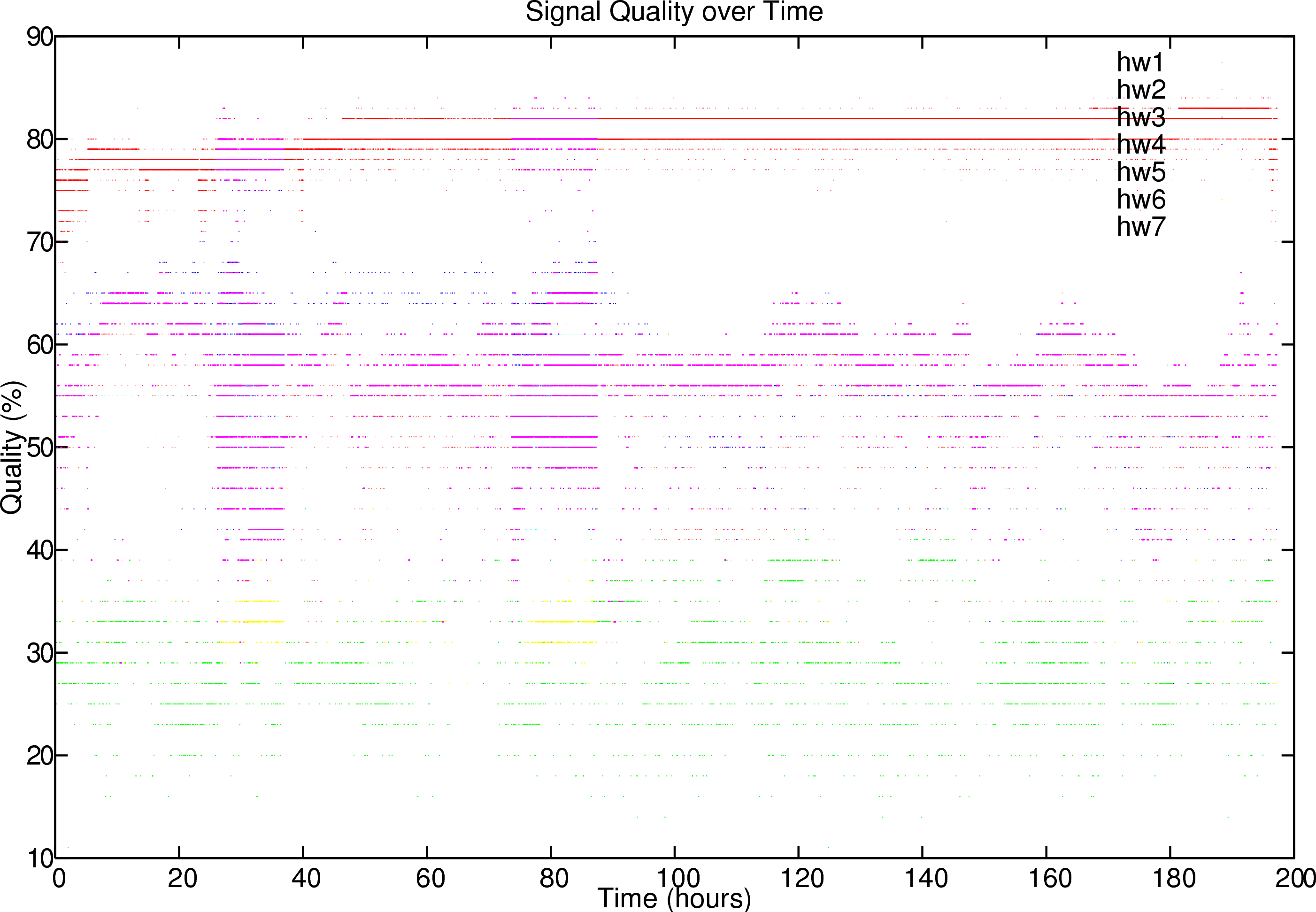
The quality of a signal is dependent on the background noise. If it is high the signal quality lowers. The sampling period started Mon Oct 23 16:50:20 CEST 2006 and ended Tue Oct 31 22:07:10 CET 2006. Every 10 seconds a sample was acquired. Figure 8 presents the results for signal level and quality. The different base station hardware addresses are listed in different colors.
4.2 Quality Variance
|
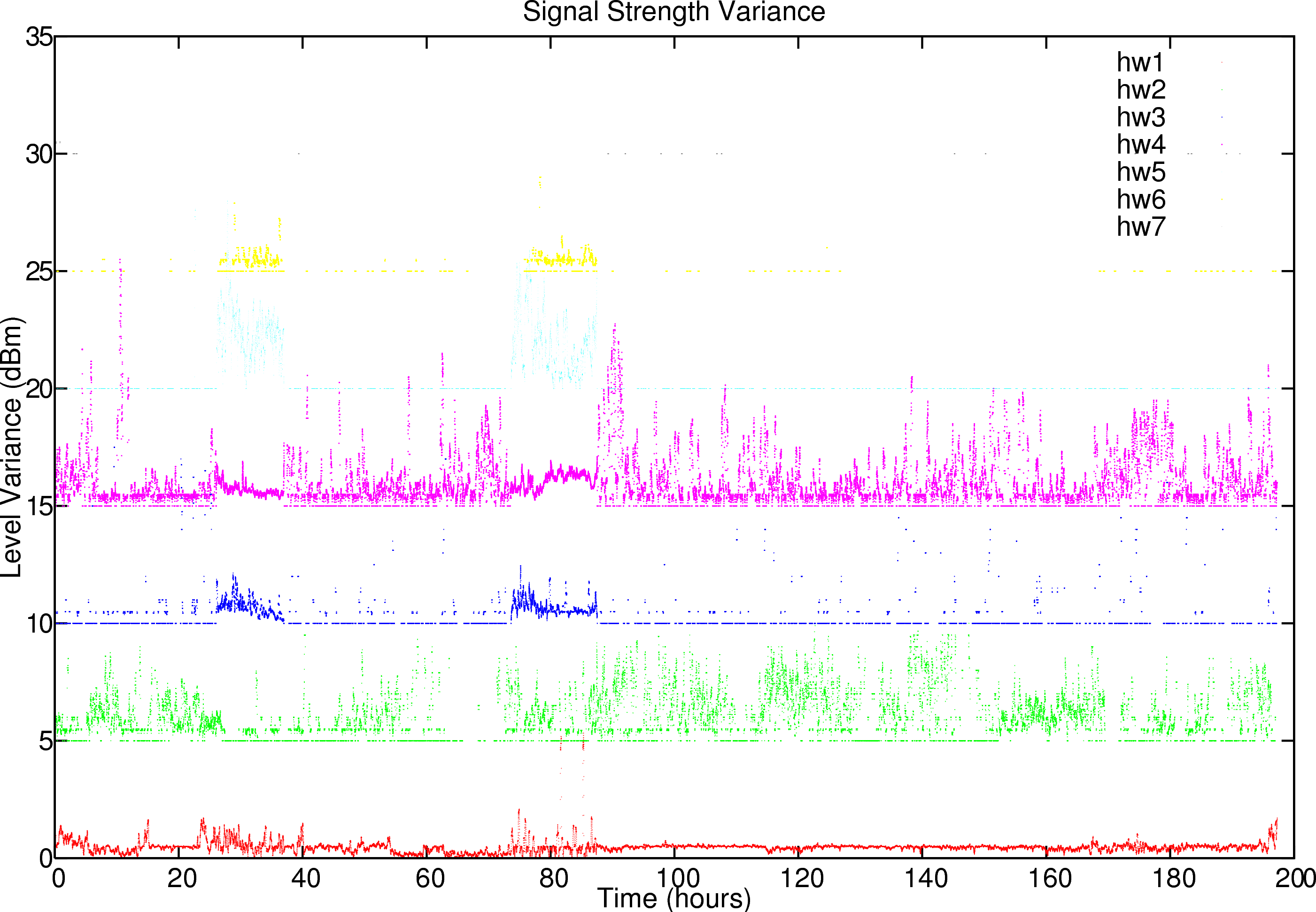
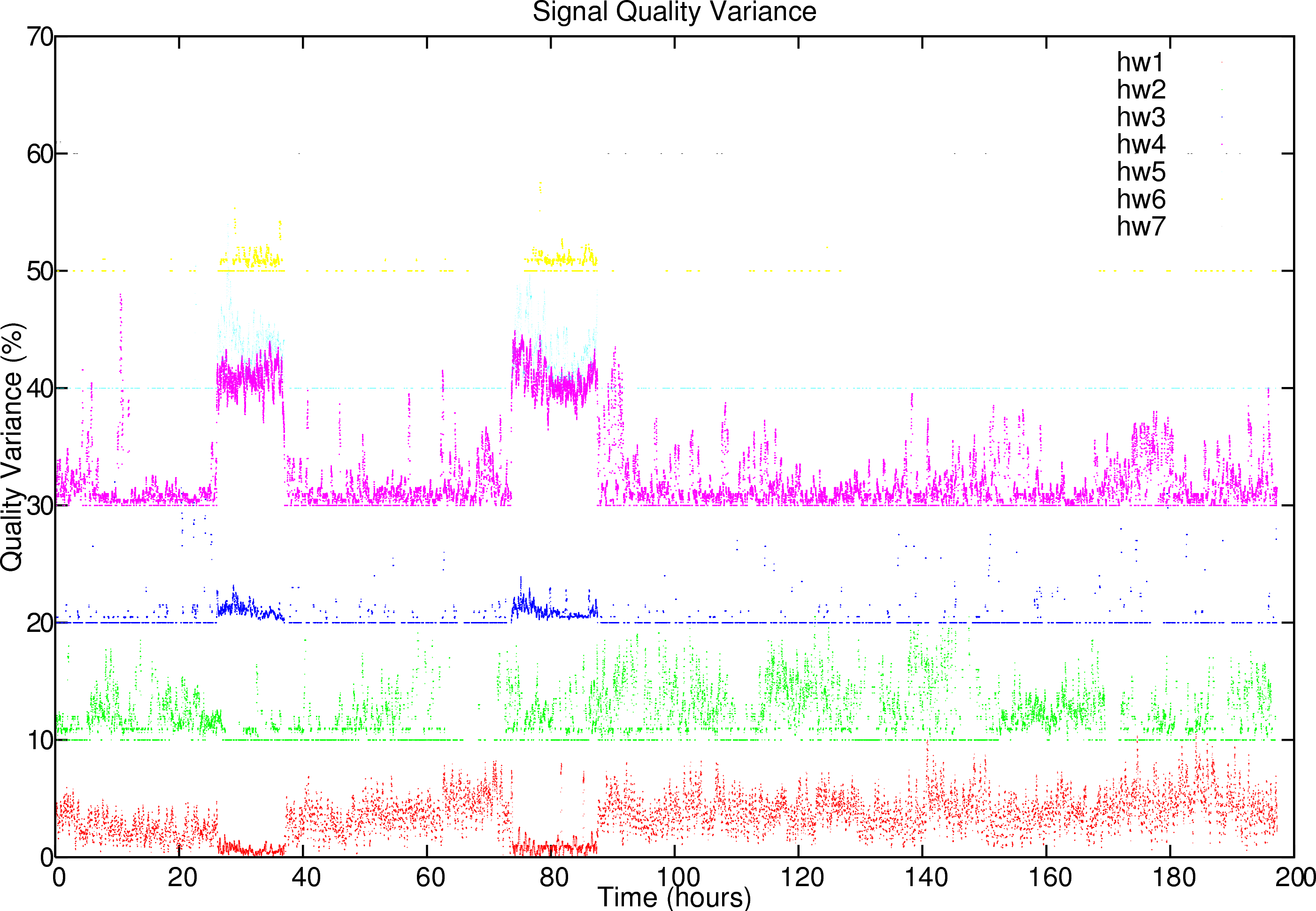
To assess upper and lower limits to the quality over a specific time we measured the absolute variance over time. These are set out in figure 9. Interestingly we find that the signal variance is relatively low, but there seems to be some cross correlation between the different base stations both regarding the signal strength and the signal quality.
4.3 Cross-linked Channels
Correlating the different data sets gives the following measures. All the values where we do not have a measurement for one of the two sets have been removed. Only dataset with more than 30 overlapping samples have been retained. Others report nan.
-
- Correlation between signal strength of different senders
hw2 hw3 hw4 hw5 hw6 hw7
hw1 -0.03 0.2 0.1 0.06 -0.003 -0.2hw2 0.1 -0.03 -0.09 -0.07 nan
hw3 0.07 0.3 -0.04 nan
hw4 0.008 0.01 -0.5
hw5 -0.08 nan
hw6 nan
Correlation between signal quality
hw2 hw3 hw4 hw5 hw6 hw7
hw1 0.1 -0.09 -0.2 -0.05 -0.05 -0.6
hw2 0.1 -0.01 -0.09 -0.07 nan
hw3 -0.1 0.3 -0.05 nan
hw4 -0.09 0.06 -0.5
hw5 -0.08 nan
hw6 nan
Correlation between signal variance
hw2 hw3 hw4 hw5 hw6 hw7
hw1 -0.2 -0.004 0.003 -0.5 -0.08 -0.2hw2 -0.03 0.05 -0.2 -0.06 0.4hw3 0.1 0.7 0.02 0.4hw4 0.05 0.02 -0.2hw5 0.06 0.2hw6 0.8Correlation between quality variance
hw2 hw3 hw4 hw5 hw6 hw7
hw1 nan nan nan nan nan nan
hw2 0.7 -0.1 -0.5 nan nan
hw3 0.9 nan nan nan
hw4 nan nan nan
hw5 nan nan
4.4 Oscillations
|
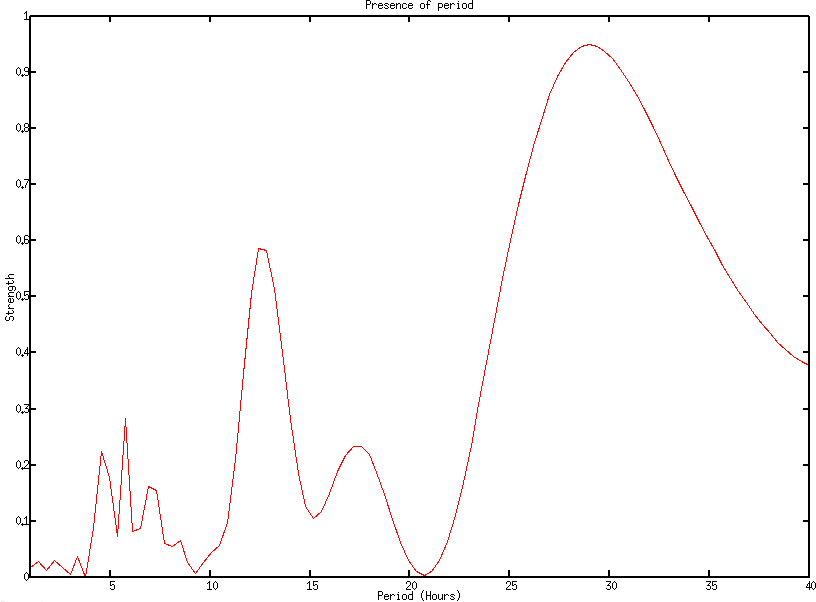
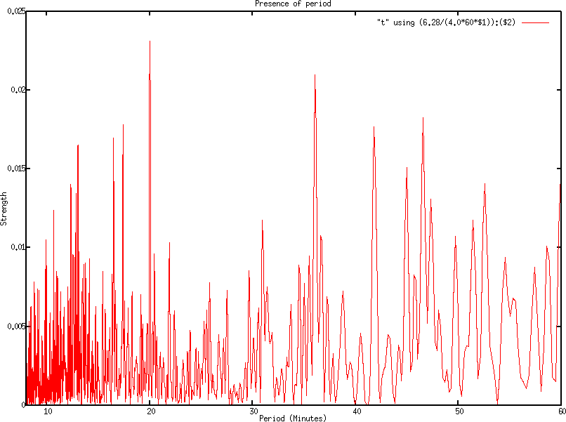
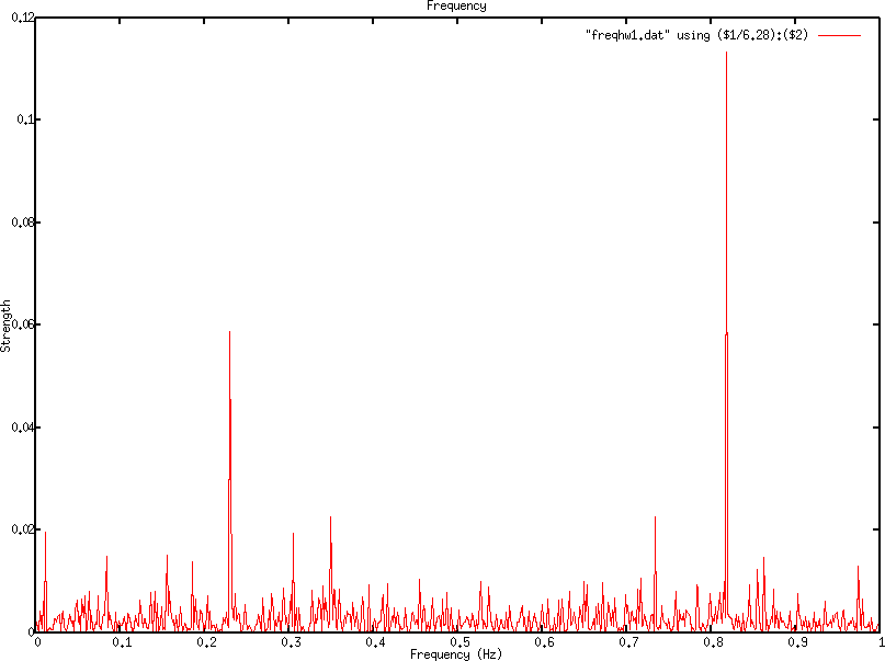
Our analysis shows multiple oscillations of the signal strength. Figure
8 and 9 already
hints that the signal quality and strength oscillates over time.
Irregular
sampling can provide us with more detailed information (above the
Nyquist frequency) [14, 15]. Using the
Lomb-periodogram,
we analyzed the oscillation of hardware address 1. Figure 10
plots the results. As can be seen, we have a strong signal strength
oscillation every ![]() hours, which
is not so unexpected. The
3daily oscillation is due to our sampling over the weekend. Looking
at the oscillation on an hourly basis we find that we have a strong
signal every 20 minutes, which coincides with the DHCP leases. At
the Hz level we indeed find that we have an oscillation around 0.2
Hz (every 5 seconds) and 0.8 Hz (every 1.25 seconds). Where these
come from is unclear. The conclusion from these small experiments
is that we need to take into account the date at which moment a signal
is sampled since it seems to relate to the signal strength.
hours, which
is not so unexpected. The
3daily oscillation is due to our sampling over the weekend. Looking
at the oscillation on an hourly basis we find that we have a strong
signal every 20 minutes, which coincides with the DHCP leases. At
the Hz level we indeed find that we have an oscillation around 0.2
Hz (every 5 seconds) and 0.8 Hz (every 1.25 seconds). Where these
come from is unclear. The conclusion from these small experiments
is that we need to take into account the date at which moment a signal
is sampled since it seems to relate to the signal strength.
5 Conclusion
In this article we investigated the possibility to model signal strength based on finding the antenna position and modeling local variations. We found out that thin plate splines are well suited to model local variations, which might occur due to specific local conditions (walls, reflections). They were however unsuited to find the position of the antenna and extrapolate outside their local environment. To resolve this we estimated the antenna position based on simulated annealing in combination with a simplex search method. This technique worked very well after renormalization of the energy landscape. The combination of both techniques yields the required model for one base station. The antenna position, specified as longitude, latitude and permeability provides an excellent tool to model the expected strength at any position, while the thin plate splines approach can interpolate a local error function.
We did not investigated the relaxation of the thin plate spline interpolation to have better estimation power under the presence of oscillations and measurement errors. We further assumed that an exponentially decaying signal (figure 7) represents a correct model. We found information documenting the possibility of a linear decaying signal [16] (last page). We also did not study anisotropic antennas. An experiment in measuring signal strength over a week long period revealed important, yet unmodeled, phenomena: crosstalk and signal strength oscillations at various periods.
Bibliography
| 1. | An Experimental Study of Localization Using Wireless Ethernet Andrew Howard, Sajid Siddiqi, Gaurav S Sukhatme Proceedings of the 4th International Conference on Field and Service Robotics (FSR'03); July; 2003 |
| 2. | Experiments in Monte-Carlo Localization using WiFi Signal Strength Sajid Siddiqi, Gaurav S. Sukhatme, Andrew Howard Proceedings of the International Conference on Advanced Robotics; address: Coimbra, Portugal; July; 2003 http://cres.usc.edu/cgi-bin/print_pub_details.pl?pubid=341 |
| 3. | Ariadne: A Dynamic Indoor Signal Map Construction and Localization System Yiming Ji, Saâd Biaz, Pandey Santosh, Agrawal Prathima MobiSys; ACM; 2006 |
| 4. | Thin Plate Spline editor - an example program in C++ Jarno Elonen URN:NBN:fi-fe20031422 http://elonen.iki.fi/code/tpsdemo/index.html |
| 5. | Approximation Methods for Thin Plate Spline Mappings and Principal Warps Gianluca Donato, Serge Belongie institution: UCSD Departmebnt of Computer Science and Engineering; number: CS2003-0764; September; 2003 http://www.cs.ucsd.edu/Dienst/UI/2.0/Describe/ncstrl.ucsd_cse/CS2003-0764 |
| 6. | Principal Warps: Thin Plate Splines and the Decomposition of Deformations. F.L. Bookstein IEEE Trans. Pattern Anal. Mach. Intell; volume: 11; pages: 567-585; 1989 |
| 7. | Interpolation des fonctions de deux variables suivant le principe de la flexion des plaques minces. J. Duchon RAIRO Analyse Numérique; volume: 10; pages: 5-12; 1976 |
| 8. | Multivariate Interpolation at Arbitrary Points Made Simple J. Meinguet J. Appl. Math. Phys.; volume: 30; pages: 292-304; 1979 |
| 9. | Spline Models for Observational Data G. Wahba Philadelphia, PA: SIAM; 1990 |
| 10. | Thin Plate Spline Serge Belongie From MathWorld - A Wolfram Web Resource; 2000 http://mathworld.wolfram.com/ThinPlateSpline.html |
| 11. | Interpolation by Regularized Spline with Tension: I. Theory and Implementation Helena Mitáavsová, Lubovs Mitáavs Mathematical Geology; volume: 25; number: 6; pages: 641-655; 1993 |
| 12. | Interpolation by Regularized Spline with Tension: II. Application to Terrain Modeling and Surface Geometry Analysis Helena Mitávsová, Jaroslav Hofierka Mathematical Geology; volume: 25; number: 6; pages: 657-669; 1993 |
| 13. | Federal Standard 1037C: Telecommunications: Glossary of Telecommunication Terms institution: United Stats General Services Administration; Federal Property and Administrative Services Act of 1949; 1949 |
| 14. | Least-squares frequency analysis of unequally spaced data N.R. Lomb Astrophysics and Space Science; volume: 39; pages: 447-462; 1976 |
| 15. | Numerical Recipes in C++ William T. Veterling, Brian P. Flannery Cambridge University Press; editor: William H. Press and Saul A. Teukolsky; chapter: 13.8. Spectral Analysis of Unevenly Sampled Data; pages: 575-585; edition: 2nd; Fenruary; 2002 |
| 16. | Lecture 3: Background on Radio Channel Maria Papdopouli institution: Department of Computer Science University of Crete & University of North Carolina at Chapel Hill; Fall 2005 http://www.csd.uoc.gr/~hy439/lecture3.ppt |
| http://werner.yellowcouch.org/ werner@yellowcouch.org |  |