| Home | Papers | Reports | Projects | Code Fragments | Dissertations | Presentations | Posters | Proposals | Lectures given | Course notes |
|
|
Enhancing Loudness and Avoiding Compressor CarnageWerner Van Belle1 - werner@yellowcouch.org, werner.van.belle@gmail.com Abstract : Explains a- the cause of compressor carnage, which is the endless stream of ticks produced by many commercial compressors. b- how a hold circuit combined with a Bessel filter can mediate this problem. c- how to efficiently implement the required attack and hold lines using the Titchmarsh convolution theorem. d- how a loudness enhancer with very short attack/decay times can be created using the above methods.
Keywords:
audio compression, loudness enhancement, compressor carnage, compressor ticks |
Table Of Contents
Introduction
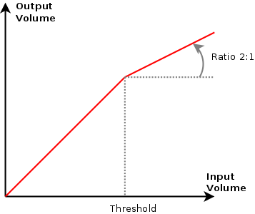 A Typical compression curve
explaining the mapping from input volume to output volume.
|
When one deals with compression, one often sees typical compression curves that explain to the layman how the input signal is mapped onto the output signal. For instance, in the above picture, When the input volume is louder than the threshold, the compressor no longer lets through the full energy. The 'ratio' of the compressor specifies how steep the angle beyond the threshold is. A 1/20 ratio means that 20 volume-units are brought back to a single volume-output. In this example the ratio is about two to one.
Normally the unit on these axes is expressed in decibels. Allthough an interpretation as RMS values might be possible as well. In our experience, compressing the sound using RMS energy levels is often perceived as being 'smoother' as one in which the compression curve is interpreted as decibels. The difference is however not that relevant in this article. Consequentyly throughout the following text, we will often switch between the two interpretations.
| ||||
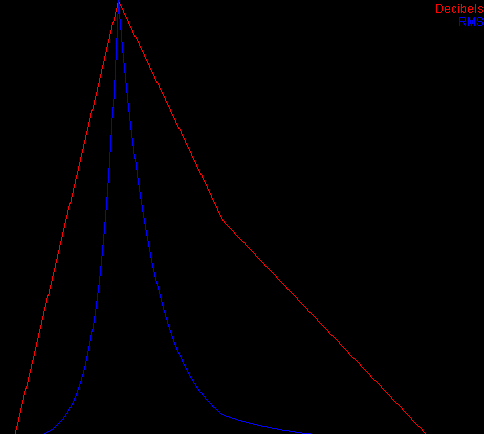
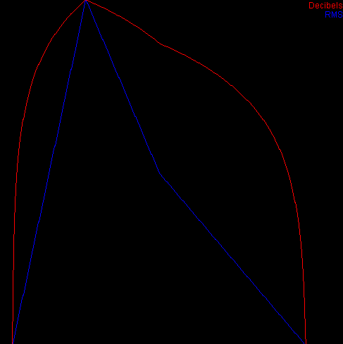
| Left: envelope calculated in decibels and then converted to RMS. The envelope calculation required a set minimal dB (e.g: -96 dB). Right: compression envelope calculated on the RMS values and then converted to decibels. |
When a linear fixed time decay is drawn on the RMS scale and then converted to decibels, we observe a highly nonlinear dB shape (see above picture).
The Problems
Attack/Decay bouncing off flanks
Compressors are often associated with an attack and decay. These make it possible to start compressing the sound before the louder volumes are truly present and to slowly come back from a strong compression.
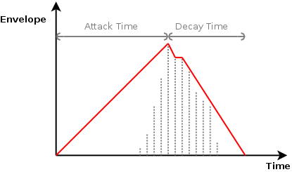 The actual RMS value is shown
as grey impulse bars. The reinterpreted energy is shown in red.
|
The decay and attack phase both rely on a slope that is added before and after the maximum energy level. How the slope behaves depends on the compressor we design. This in turn depends on the unit we use on the envelope axis. Although, from the above discussion it might appear natural to use dB, it is also problematic because we cannot easily represent zero energy and at very low energies we obtain fairly large absolute dB values. So in a sense, it might be more valuable to work directly on the measured energy.
A Linear, Time dependent Slope
With a linear, time dependent slope we calculate an appropriate deltavalue that will allow us to reach the target value (0 energy) within T samples, starting from the maximum value that triggered the compression. This delta is then used to draw an envelope in front (an attack) or behind (a decay) the largest energy.
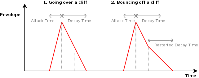 When during the decay phase
the energy levels are somewhat too large, a new decay phase is set in,
but with a different slope.
|
This strategy has the drawback that the attack/decay phase can 'bounce off' of flanks (as pictured above). This means that silent sounds will have smaller volume changes than loud ones, because the slope is calculated based on the local maximum (for silent passages, this maximum value is small, thus the angle will be small as well). It might appear that this is wanted, however, when in the middle of a bassdrum that is being made louder, suddenly stopping and reorienting to a lower compression ratio will lead to audible unwanted artefacts.
A Linear Fixed Delta dB Slope = An Exponentially Decaying Energy Slope
The biggest problem of the previous strategy is that the decay curve can 'bounce off' of flanks that are just a tiny little bit above the threshold. We don't really like that because it introduces behavior that is often difficult to track/understand. To overcome this problem it is possible to force the decay rate to be the same (e.g: -0.03 dB/sample), independent from the local maximum that was the ankerpoint for the attack/decay.
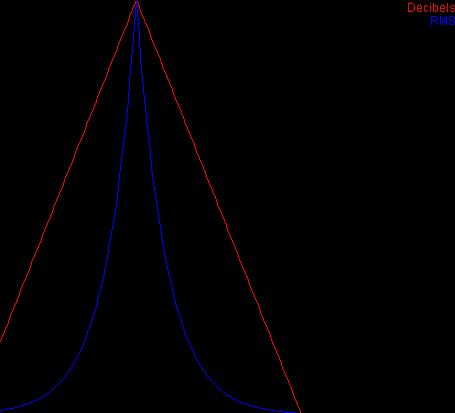 A Linear decaying decibel slope implies
an exponentially decaying energy slope
|
The advantage of this strategy is that we no longer bounce off the flanks. The perceived volume change is the same, independent of the starting point of the decay/attack.
In a dB scale this means that we draw linear lines, all with equal slope. On the RMS scale this behavior can be quickly implemented using a single multiplication for each sample, which is a lot less computational expensive than going over a logarithm and exponential. For instance: multiplying each sample with 0.999 would mean a -0.008690235 dB loss per sample (20*log(0.999))
Personally I prefer this strategy since it is the most intuitive, and when computed on the energy levels, it is fast and also works on negative values, which is sometimes wanted.
The drawback on the other hand is that it is difficult to specify an attack/decay time, since we mainly work with a halflife time (just by multiplying energy levels we will never reach 0). This problem translates itself further into a problematic specification of the buffersize of the attacks' delay line. Because the energy level of the attackenvelope will never reach zero, it is theoretically impossible to use a fixed delay line to look into the future.
An easy solution to deal with this is to set the minimum energy to which we are still sensitive (E.g: -96 dB should suffice when dealing with 16 bit data) and to specify a maximum value. Based on those two values one can determine the necessary length for the delay line.
Another possible solution is to use a distorted exponential envelope for the attackpahse. Thereby we could ensure that the attackenvelope always crosses zero after a certain timespan.
Envelope Discontinuities
We saw that an improper (but natural) implementation of an attack/decay line can lead to unwanted artefacts. There are however some other artifacts that also deserve some attention. The ones described below can readily be observed in a lot of commercial music [1] and all stem from the same source: discontinuities in the envelope calculation. This is especially important when dealing with short attack/decay times. In those instances it is very well possible to create a string of ticks and small breaks in the waves as we process them. This leads to audible artifacts and distorted waves, as often heard in many overly compressed songs.
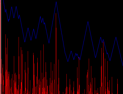 Linear Attack Decay curves
introduce discontinuities in the audiostream. The red line represents
the original audio, the blue line the envelope. The envelope appears
to lie above the curve due to a limitted plot accuracy. Each peak in
the blue line corresponds to a peak in the audio
|
It is worth noting that the problem visualized above, cannot be solved by introducing a 'knee' into the compression curve because the switch from decay to attack is sudden and can happen as well below the knee point. Also an application of RMS-multiplication instead of energy-deltas does not solve the problem.
Wave Shape Alterations
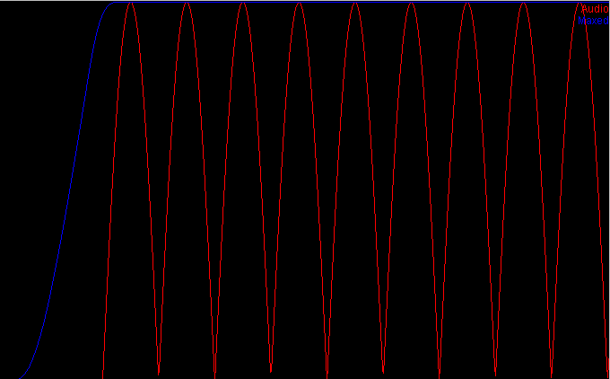
Another aspect to short attack/decay times is that they might introduce waveshape modifications, and thereby introduce harmonics. The following picture demonstrates a sine wave at 20 Hz, the estimated energy and the resulting changes to the sine wave.
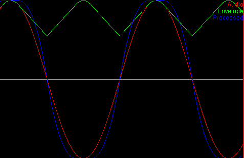 Demonstration on how
compression can modify the waveshape and introduce harmonics.
|
It is worth pointing out here that the above waveform alteration has nothing to do with digital clipping. The waveshape changes because the envelope engulfs it with a similar shape. The multiplication of these two shapes then leads to a new shape, with different harmonic characteristics.
Solving these Problems
Hold and Smooth
To avoid the two above mentioned problems it is useful to introduce a hold function which will hold the maximum over a certain period of time, before falling into the decay phase. The problem of discontinuities can then best be solved by applying a lowpass filter on the envelope curve. This smoothens any discontinuities and, when set up correctly, will also ensure that the envelope never falls below the actual audio.
Implementation: the fastest method I found to solve the two problems at once is to spread out local maximum values and then apply a Bessel filter [2, 3]. A Bessel filter is a fast lowpass filter that has the most constant group delay [4, 5] in the bandpass region (at least with respect to elliptic filters). Thus, adding an appropriate delay time should realign the input and the envelope.
| ||||
| The envelope after performing a max-hold and Bessel filtering will never fall below the absolute value of the input data. |
Efficient Attacks
Implementing a decay is fairly straightforward. With every new step, we decrease the current decay using a term (multiplier) or factor (delta). Afterward, we check whether the decay is larger or smaller than the incoming sample. If the new sample is larger, then the decay is set to this value.
The implementation of an attack is similar, except that one performs it backwards. In realtime systems this poses a problem because we cannot predict what is about to come. In a sense one must go back in time and draw the envelope before the recently found maximum. To create such acausal system, a delay line can be used because it offers us the necessary look ahead and a way to overwrite the past. With a delay line we can effectively modify the values that we would have returned if we had known the new incoming value. Every time a new sample comes in, the attack is processed as a backward decay through the delay line. A parallel delay line then keeps track of the incoming samples such that the envelope and the audio signal are properly aligned.
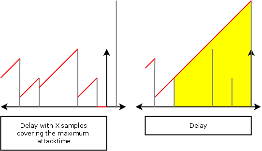 Left: two delay buffers. The
first containing the envelope (red values). The second containing the
samples we have seen (gray values). Right: As soon as a new value
comes in, it is placed in the sample-delay buffer and calculated
backwards through the envelope buffer. The yellow area is the area
that we had to investigate for this single incoming sample.
|
This is an overall expensive operation. For large attacktimes we might end up processing the entire delay buffer for every individual sample, requiring 'buffersize' operations per sample. This can be solved by looking at more than one sample at a time. Then it is possible to process the input in reverse and with the outgoing 'backward' decay, we continue to process the data in the delay buffer.
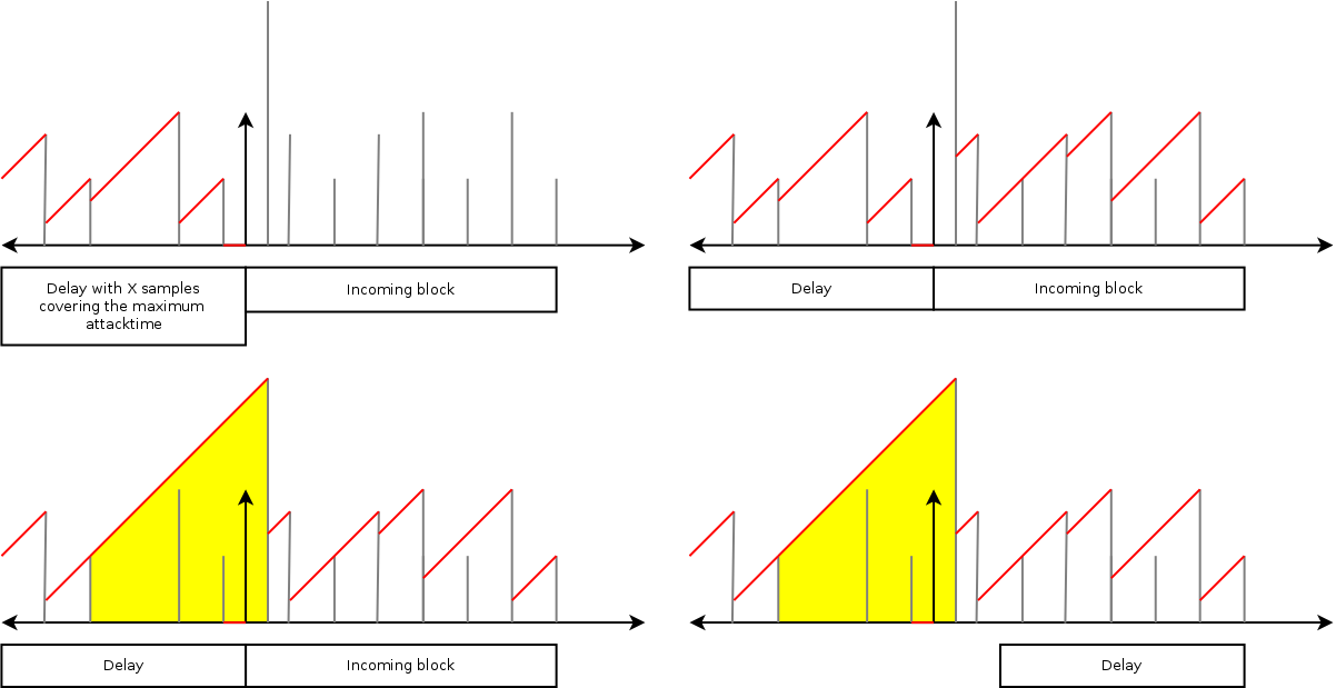 Top left: the startphase with
envelope (red) and sample (grey) buffers. Top right. When a new block
comes in, we first process the envelopes of the new block from right
to left. Bottom left: once we reach the boundary of the delay buffer,
we propagate the decaying value through the envelope buffer as
well. Bottom right: finally we move all buffers to their new
positions.
|
Efficient Holds
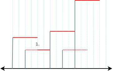 Holding the last seen maximum for
about 4 samples. The input samples are drawn in grey. The full red
line shows the hold result. The dotted red lines the result that could
have been if it was not overridden by another maximum.
|
A hold line is one in which we remember the current maximum for a limited amount of time. This is demonstrated in the above picture where a list of values produced an envelope where the latest (since 4 samples ago) maximum is retained. Such a hold circuit can be used to create a prehold or a posthold, depending on the delay time of the parallel sample circuit. For instance. If we would process the hold line and then delay all (gray) samples with 4 ticks, we would have created a prehold. Below we will therefore only focus on a post-hold, which is already more than complicated enough.
At first sight, the problem appears similar to the attack problem. With an appropriate buffer, we can always go back in the past and overwrite the samples that have been seen already. Consequently, we could assume that a similar block based setup would speed up the algorithm when dealing with larger inputs. Unfortunately, that's not the case. The main reason for that is that an attack (or reverse decay) comes naturally to an end when its value becomes smaller than the test sample. And this will always be reached before the end of the delay buffer because our attack/decay value will cross the zero line there. A hold line does not have such automatic stop and must rely on an internal counter to know when it should stop. At that point, it also does not know anymore what the new 'latest' maximum would have been. This is illustrated in the above picture: at the first drop of red (labeled number 1.), the red line continues 2 units lower because during the hold phase we saw a secondary maximum that would take over as soon as the old was held sufficiently long. Keeping track of all these submaxima forms a serious time consuming problem, and would without further optimization, force us to investigate every single sample and its full neighborhood.
Luckily there is something useful that we can observe. Namely that whenever we continue after a maximum came to an end, we will continue with lower values. Actually, with each new step, we will continue with lower values until we reach a new larger maximum. Thereby, any valleys (a local minimum followed by a local maximum) that appear under the drawn maximum will not appear in the exit segment. (If this sounds confusing, don't worry: it is confusing, but nowhere near some axioms we might be referring to such as Titchmarsh convolution theorem [6]).
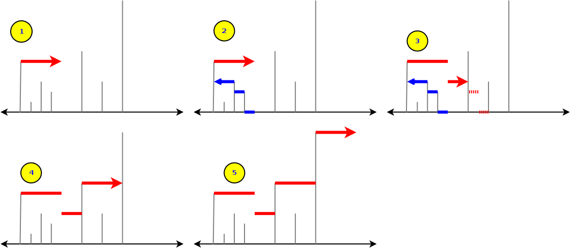 A faster implementation of a hold
maximum algorithm. It works in two phases: a- A forward hold calculation
and b- an exit segment (blue) calculation).
|
The presented algorithm works in a number of phases.
- Continue from left to right (1). Accept new maximum-values as we encounter them. If no new maximum is encountered increase a hold counter.
- When the hold counter reaches its timeout, we go back in time to create the 'exit' segment (2). This is done by retaining the last maximum starting at 0. When the start of the exit segment is determined (the blue line),
- we start drawing it after our exit point (3). We do this until an incoming sample is larger than what we are drawing, or until the exit segment is fully drawn. Once done, we go back to step 1 (On figure 4 & 5).
Even more efficient holds
About eleven motnhs after writing this article I found an interesting article by Daniel Lemire [7]. It describes a system to perform min/max hold in streaming mode with about 3 operations per sample. A truly ingenious algorithm.
Conclusion
Compressors are tricky beasts to write correctly
- The envelope calculation should avoid bouncing off flanks by relying on a fixed decibel slope (or exponential RMS slope).
- The envelope should be a continuous function. Discontinuities should be smoothened out with an appropriate lowpassfilter.
- The envelope should not stretch around the energy peaks, instead it should lay above it, otherwise harmonics are introduced. A hold circuit that spreads the maximum back around the peaks is useful to solve this.
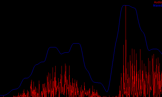
 A loudness enhancer
using a attack/hold/decay line and Bessel filtering of the
envelope.
|
An efficient algorithm to hold the maximum over a certain timespan was presented, as well as its application together with a Bessel filter to create a fast acting limiter.
Acknowledgments
Nancy Gerits for proofreading this text.
Bibliography
| 1. | The Death Of Dynamic Range Bob Speer CD Mastering Services http://cdmasteringservices.com/dynamicdeath.htm |
| 2. | Delay Networks having Maximally Flat Frequency Characteristics W. E. Thomson Proceedings of the Institution of Electrical Engineers, Part III, November 1949, Vol. 96, No. 44, pp. 487–490. |
| 3. | Electronic filter simulation and design Giovanni Bianchi, Roberto Sorrentino McGraw–Hill. pp. 31–43; 2007 |
| 4. | Group Delay Distortions in Electroacoustical Systems J. Blauert, P. Laws Journal of the Acoustical Society of America 63 (5): 1478–1483; May 1978 |
| 5. | Discrete-Time Signal Processing Alan V. Oppenheim, Ronald W. Schafer Prentice Hall; editor: John R. Buck; 1989 |
| 6. | The zeros of certain integral functions Edward Chalres Titchmarsh Proceedings of the London Mathematical Society 25: 283–302; 1926 |
| 7. | Streaming Maximum-Minimum Filter Using No More than Three Comparisons per Element. Daniel Lemire Nordic Journal of Computing, 13 (4), pages 328-339, 2006 http://arxiv.org/abs/cs.DS/0610046 |
| http://werner.yellowcouch.org/ werner@yellowcouch.org |  |
