| Home | Papers | Reports | Projects | Code Fragments | Dissertations | Presentations | Posters | Proposals | Lectures given | Course notes |
|
|
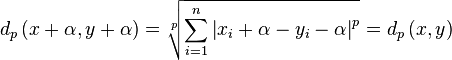
On distances between energy vectorsWerner Van Belle1* - werner@yellowcouch.org, werner.van.belle@gmail.com Abstract : An audio-vector describes for each frequency band how much energy we find at a specific position. In this paper we investigate the problem of comparing audio-vectors. We present a new method to compare real or complex energyvectors.
Keywords:
energy comparison, psychoacoustics |
Table Of Contents
Introduction
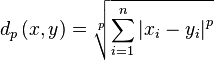
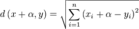
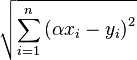
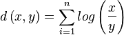
A distance between two energy vectors can generally be written as follows
RMS
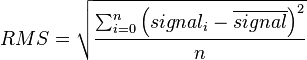
The first common energy representation is an RMS value, or the root means square, defined as
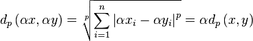
When the signal volume is increased with a gain of
 , then the RMS value will be multiplied by
as well.
, then the RMS value will be multiplied by
as well.
When comparing RMS values with a normal  metric, we can describe the effect of a gain modification to both
vectors as follows.
metric, we can describe the effect of a gain modification to both
vectors as follows.
Thus the distance between two vectors increases if we increase their volume. Acoustically this is wrong because they are qualitatively still exactly the same tracks.
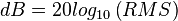
dB
The second common description of energy is the log value of the
RMS; in audio typically described as dB and defined as
 . A volume increase of
the signal results in an addition to the log value. A gain
modification to both vectors has no effect on the resulting
distance.
. A volume increase of
the signal results in an addition to the log value. A gain
modification to both vectors has no effect on the resulting
distance.
A desirable property. Yet, we now have the problem that when an
underlying RMS value becomes very small, its logarithm becomes
unreasonably large. It can even be  . We find
that the overall distance is dominated by the
values that represent the most silent part of input
signal. Acoustically this is wrong.
. We find
that the overall distance is dominated by the
values that represent the most silent part of input
signal. Acoustically this is wrong.
Observation 1: the two most commonly used energy representations
are acoustically wrong.
- The distance between RMS vectors increases when the volume of the two vectors increases.
- The distance between dB vectors is dominated by the most silent
contributions of the signals.
Normalization schemes
Of course, it is not sufficient to be robust against a volume modification on both input channels. In practice, we must be invariant towards a volume change of either input signal. A standard approach to this problem is to normalize the input vectors.
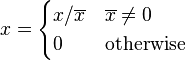
Division by the average
When dealing with RMS values, a division by the average would normalize the input vectors appropriately. The normalized vector is given as
With such normalization the distance between two RMS vectors would satisfy our requirement:
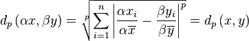
And although this normalization strategy guarantees volume
invariance, it does not find the optimal for which
 will be the smallest. First we give a
demonstration of this in L1
will be the smallest. First we give a
demonstration of this in L1
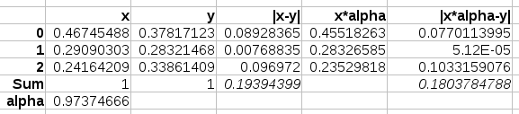 In the above
demonstration we have two 3 dimensional vectors, both normalized
at a sum of 1. Their L1 distance is computed as 0.1939, however
a closer distance is possible when \alpha is chosen as 0.97. In
that case their distance is 0.1803.
In the above
demonstration we have two 3 dimensional vectors, both normalized
at a sum of 1. Their L1 distance is computed as 0.1939, however
a closer distance is possible when \alpha is chosen as 0.97. In
that case their distance is 0.1803.
|
In a large test we conducted, the average error between the minimal distance and the distance through normalization was about 5.3%
Now will give a demonstration that also in L2 such normalization
will not find the optimal for which
 will be the
smallest. Important here is that this type of normalization is similar
to normalizing the width of the distribution if x and y were vectors
describing the distance to the mean. (In which case we would have
normalized the standard deviation, which is a very common
approach).
will be the
smallest. Important here is that this type of normalization is similar
to normalizing the width of the distribution if x and y were vectors
describing the distance to the mean. (In which case we would have
normalized the standard deviation, which is a very common
approach).
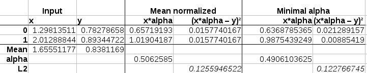 In this demonstration
we work with 2 dimensional vectors. In the first instance we determine
the \alpha ratio by dividing the means of y and x. The result is a L2
distance that is 0.1256. The minimum distance would however be 0.1228
at an \alpha=0.49061.
In this demonstration
we work with 2 dimensional vectors. In the first instance we determine
the \alpha ratio by dividing the means of y and x. The result is a L2
distance that is 0.1256. The minimum distance would however be 0.1228
at an \alpha=0.49061.
|
Observation 2: dividing an RMS vector by its average does not help us to find the minimum distance between them if the volumes of the vectors is allowed to change.
Subtracting the average
For log values we could consider subtracting their average before comparing them:

Regardless of the volume of any of the inputs, they will always be brought to the same level when comparing them.

This normalization method will report the same distance as
 . And it is also the basis
for least-squares optimization. It does however stop there, and this
normalization does not work in L1 as is demonstrated in the following
example.
. And it is also the basis
for least-squares optimization. It does however stop there, and this
normalization does not work in L1 as is demonstrated in the following
example.
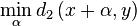
 The above example
shows how a normalization through subtracting the average will not
lead to a minimal distance of the L1 distance. The correct distance is
3.208 at a volume change 0.252. Yet, after normalization we find a
distance of 4.1100.
The above example
shows how a normalization through subtracting the average will not
lead to a minimal distance of the L1 distance. The correct distance is
3.208 at a volume change 0.252. Yet, after normalization we find a
distance of 4.1100.
|
Observation 3: subtracting the average from a dB vector is only a valid normalization scheme if we use an euclidean distance to compare them.
Minimum L1 distances
Let's recap: dB representations are dominated by the silent parts of the signal. And for the RMS representation we have no volume normalization that actually works.
We will now discuss how we can find the minimum distance in L1
between two vectors, first assuming that we have a volume term (add
), afterwards assuming that we have a volume factor (multiply
with ).
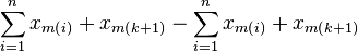
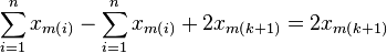
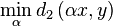
Minimum distance between vectors with additive volume
Given two vectors x and y, and a metric L1. What scalar should we subtract/add to the coordinates of x to minimize 
This value is minimized when 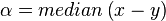 . Thus we have

The performance of this approach:  to find the median, and
  to calculate the sum.
At this point it might be tempted to assume that we could still get away with normalizing the individual vectors by subtracting their medians, yet that will not work because 
 The example above has two 4-dimensional points. The median of x is 0.63. The median of y is 0.456. If we subtract the median values from respectively x and y, and then calculate the L1-distance, we have a value of 3.35. If, on the other hand, we subtract the values, calculate the median, and subtract it within the distance calculation we get a distance of 3.2088.
|
Observation 4: the L1 metric for dB values can be minimized by subtracting the median of the differences within the distance calculation.
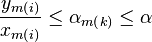
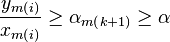
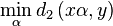
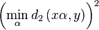
Minimum distance between vectors with multiplicative volume
Given two vectors x and y, we look to minimize the L1 distance between them by allowing a scaling factor. We thus search for

|
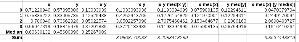
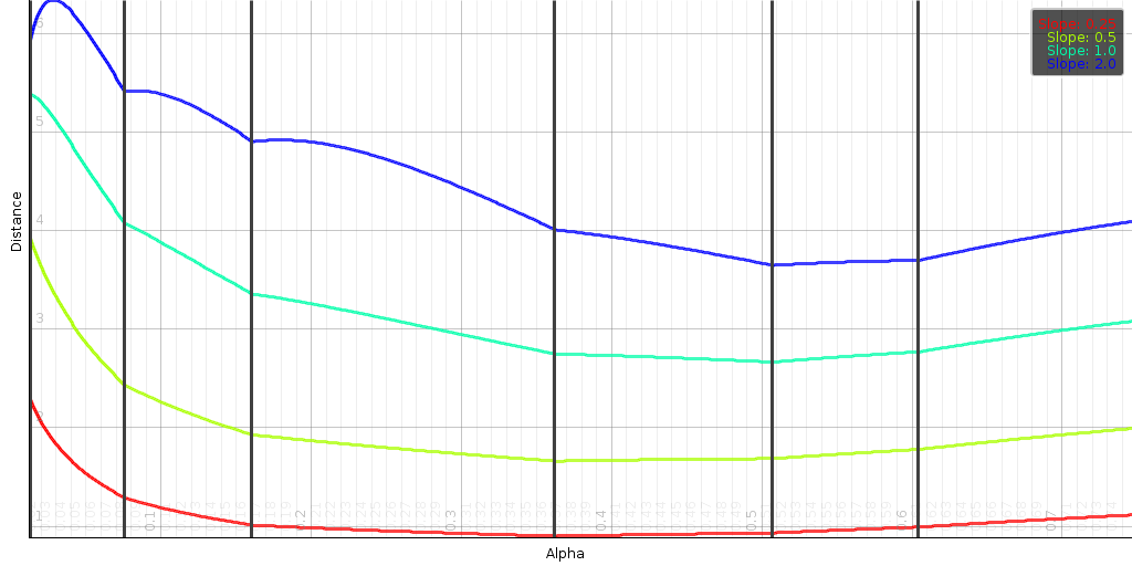
To demonstrate how the search space looks like, we created a couple
of 7 dimensional random vectors and determined the minimum and
maximum alphas (located at
 and
and
 ). Within that range we calculated
  . Clearly the curve that is being drawn is
convex. Its corner points are at
. Clearly the curve that is being drawn is
convex. Its corner points are at
 (which we drew as
vertical black lines).
(which we drew as
vertical black lines).
Finding the global minimum in such an object through standard
optimisation algorithms is fairly difficult because the function
 is piecewise linear. Its
derivative is piecewise constant. And the second derivative is 0,
except at the corner points. Consequently Newtons method is not
applicable, and a gradient descent will either be way too slow over
poorly sloped lines, or jump directly out of the box to never come
back. Luckily because the object is so well shaped it is easy to
find a fast solution.
is piecewise linear. Its
derivative is piecewise constant. And the second derivative is 0,
except at the corner points. Consequently Newtons method is not
applicable, and a gradient descent will either be way too slow over
poorly sloped lines, or jump directly out of the box to never come
back. Luckily because the object is so well shaped it is easy to
find a fast solution.
In order to do so we first prove that
is piecewise
linear.
Proof: We sort the corner points in increasing order through
mapping m (such that m(1) is the smallest and
m(n) the largest). A reordering of the terms of the summation does not
change the outcome, we can thus write:
| Equation starteq: | 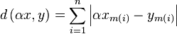 |
For any  , we will show that
is linear between
, we will show that
is linear between
 and
and
 . We do so by splitting
eq. starteq at segment k.
. We do so by splitting
eq. starteq at segment k.
| Equation split: | 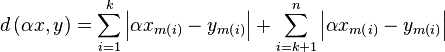 |
We are only interested in this function for
 .The
first summation has
.The
first summation has  . Therefor we have
 . From
that it follows that
. From
that it follows that  . And we can thus remove the absolute
value. For the second summation we have that
. And we can thus remove the absolute
value. For the second summation we have that  and thus
 . From
that it follows that
. From
that it follows that
 . We can
rewrite [eq:split] as
. We can
rewrite [eq:split] as
|  |  |
 |
which is indeed a linear equation in .
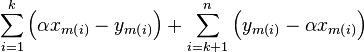
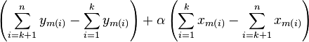
A second observation is that each segment has a higher slope than the previous one. To see this, compare the slope of segment k+1 against the slope of segment k
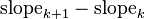 | | 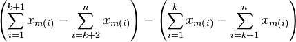 |
|  | |
|  |
Finally, the minimum of the overall function is given at the place
where the derivative is 0, or in our case, since the function is
piecewise linear, where the derivative switches sign. To find that
minimum, we only need to know one more thing: the start slope, which
is given at an 
| Equation startslope: | 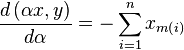 |
With the starting slope easily computed
(equation [eq:startslope]) and the slope
change given as  we can iterate
over all corner points and report the value to
be used to compute the minimal distance. This algorithm requires a
computation of all corner points
, a sorting of them
we can iterate
over all corner points and report the value to
be used to compute the minimal distance. This algorithm requires a
computation of all corner points
, a sorting of them
 and a series of
additions to find the best . Overall performance:
.
and a series of
additions to find the best . Overall performance:
.
    float determineAlpha(float[] x, float[] y)
    {
        float slope=0;
        int nextWrite=0;
        for(int i = start ; i < y.length; ++i)
        {
            float x=x[i];
            float yv=y[i];
            if (x==0) continue;
            alphas[nextWrite]=yv/x;
            float abs=Math.abs(x);
            slope-=abs;
            slopeChanges[nextWrite++]=2*abs;
        }

        QSort.inPlace(alphas, slopeChanges, nextWrite);

        float alpha=0;
        int k;
        for(k = 0 ; k < nextWrite; )
        {
            if (slope>=0) break;
            alpha=alphas[k];
            float delta=slopeChanges[k];
            while(++k<nextWrite && alphas[k]==alpha)
                delta+=slopeChanges[k];
            slope+=delta;
        }
        return alpha;
    }

    float distanceWithMinimizingRatio(float[] x, float[] y)
    {
        final float alpha=determineAlpha(x, y);
        float dist=0;
        for(int i=0;i<y.length;++i)
            dist+=Math.abs(y[i]x[i]*alpha);
        return dist;
    }
In the above algorithm, the mapping m is implicit because we sort
both the values together with their associated
slope changes. QSort.inplace(a,b,l) sorts the first l elements of
array a and b in accordance with the value in a. The algorithm deals
with 0's as follows:
-
 ,
,  . In that case
  and the change of sign when crossing the point is
-
 , . In that case
  and the change is simply
 - ,
 . In that case
  or
or  . It is however irrelevant because the slope change (positioned at an infinity) will never occur anyway.
-
 . This is a case that we do not add to the sorting list either. The points match and there is nothing we can do to not match them. So we can safely ignore this value. Or to be correct: add 0 to the starting sign.
Aside from properly dealing with 0 values, we also had to deal with consecutive \alpha_{i} values that are the same.
Observation 5: we have a lovely algorithm to find 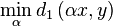 . Wiehie !
Minimum L2 distances
Minimum distance between vectors with additive volume
Given two vectors x and y, and a metric L2. What scalar should we
subtract/add to the coordinates of x and y to minimize
This value is minimized when
 , which can be realized by
subtracting the mean from x and y separately. Thus with L2 distances
we can normalize the individual vectors.
, which can be realized by
subtracting the mean from x and y separately. Thus with L2 distances
we can normalize the individual vectors.
Observation 6: subtracting the mean from the vectors is a
suitable normalization scheme to find
.
Minimum distance between vectors with multiplicative volume
Is there an easy solution to find
 ?
?
 | |  |
 | 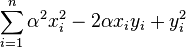 |
The distance is a quadratic equation. Its differential is
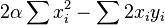 | |  |
| |  |
Somewhat of an unexpected result. This seems more like maximizing a correlation than bringing x to the level of y.
Ratio distance on real energy vectors
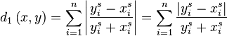
Because RMS values suffer from the problem that high frequencies are perceived louder than their values would reveal, we could consider using dB values, yet that approach has the problem that low values incur a large penalty. A solution that lies in between is to represent the vectors using their energy but limit the maximum distance two values can lay apart. In that case a rudimentary distance (without limiting) would be
A positive aspect of this is that it is volume invariant
 . In practice this means
that if we compare energy-vectors representing sound spectra, we won't
need to normalize the high frequencies such that they have a similar
'weight' as the typical louder low frequencies.
. In practice this means
that if we compare energy-vectors representing sound spectra, we won't
need to normalize the high frequencies such that they have a similar
'weight' as the typical louder low frequencies.
Next, we slap a limiter against it. From an acoustic perspective this makes sense because we will only hear the loudest of the two sounds. Whether energies are then 120 or 126 dB apart from each other, it really doesn't matter: they are unmatched.
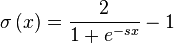
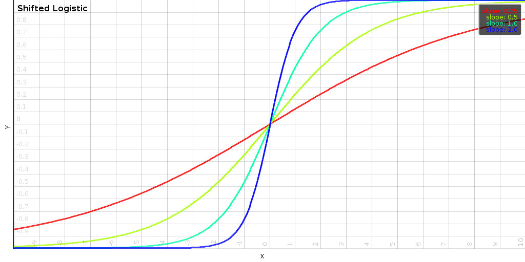
One of our favorite limiters in this case is the logistic function, which we modified to be odd. It behaves linearly around 0 but if we get to 24dB, we start to clamp the output value.
|
If we then stick our logarithmic comparison into the logistic we get the following:

which is interesting because it all suddenly became easier to compute: we lost the logarithm and we lost the exponential. And we can even simplify it further to

When s=1 it is even easier to calculate.
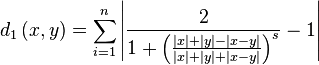
The full distance is defined as
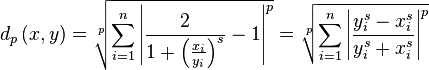
It satisfies  and is volume invariant. Furthermore, this distance function has an
upper limit
and is volume invariant. Furthermore, this distance function has an
upper limit  .
.
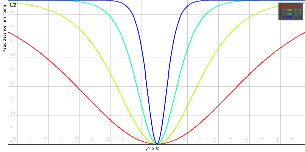
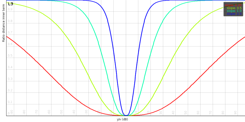
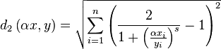
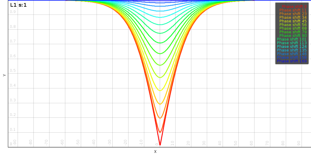
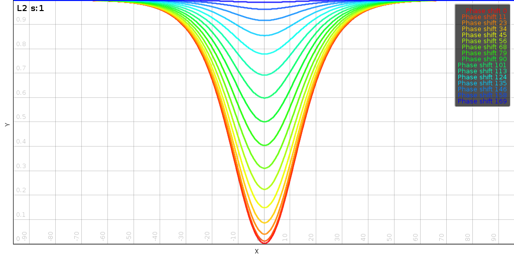
| ||||||
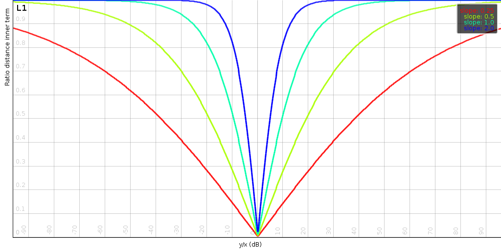
| The above plots shows the impact of the slope s and the order p of the distance. Generally, the slope determines at how many dB we start to limit the effect of a mismatch. The order determines how sensitive the distance is to small changes when two signals match. |
Optimal solutions in L1 tend to be sparse. That is: a few outliers
are allowed if we can match the rest. With that we have a distance
measure that can be blind to glaring mistakes, as long as the rest
matches. Sometimes this can be useful. L2 is related to an Euclidean
distance and is easier to interpret geometrically. Aside from the
qualitative differences on the solution, also finding the solution
requires different minimization approaches. In the following sections
we investigate the behavior of this distance in L1 and L2 and try to
find solutions to obtain 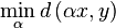
In L1
|
In L1 we have a similar result as in
section [l1-plain]: namely the optimal value
will be an element of the corner points
. The above plot shows
the function between two 7 dimensional points x and y. Each line shows the distance
function at a varying slope values. Sadly, the function
is no longer piecewise
linear.
To find the minimum distance, we try all corner points
 and report the smallest one back. This
approach has a quadratic performance, and that might be slow when n is
large. However, the terms of the summation are easily processed (after
preprocessing, essentially two sums, an absolute value and a
division).
and report the smallest one back. This
approach has a quadratic performance, and that might be slow when n is
large. However, the terms of the summation are easily processed (after
preprocessing, essentially two sums, an absolute value and a
division).
Minimzation methods such as conjugate gradient or simple gradient descent do not work well in this setting because they generally just jump off a cliff.
In L2
In L2, the distance function tends to be a lot smoother.
|
The above plot shows for varying values of s for two fixed 7 dimensional vectors. The
corner points no longer align with the actual minima. And as the slope
increases we start to find many more local minima.
To find a solution to this problem Newtons method is particularly
suited. When s is low it find the global minimum in about 2 steps. If
s is large then we start to have many local minima and finding the
correct one might require actually scanning the range from the lowest to the highest
.
Robustness of the ratio-distance
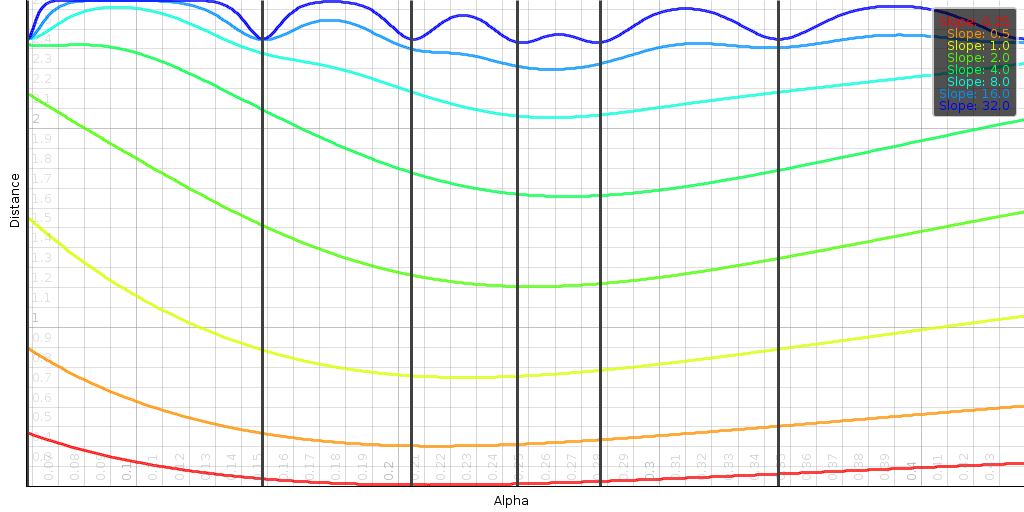
A feature of this distance is that it is robust towards a variety of features that one might consider. To demonstrate that we will use two vectors (f and g), which will gradually change from one to the other (given by parameter p). For each pair along this trajectory we compute the L1 distance, the minimal L1 distance (allowing some scaling) and the minimal L1 ratio-distance.
|
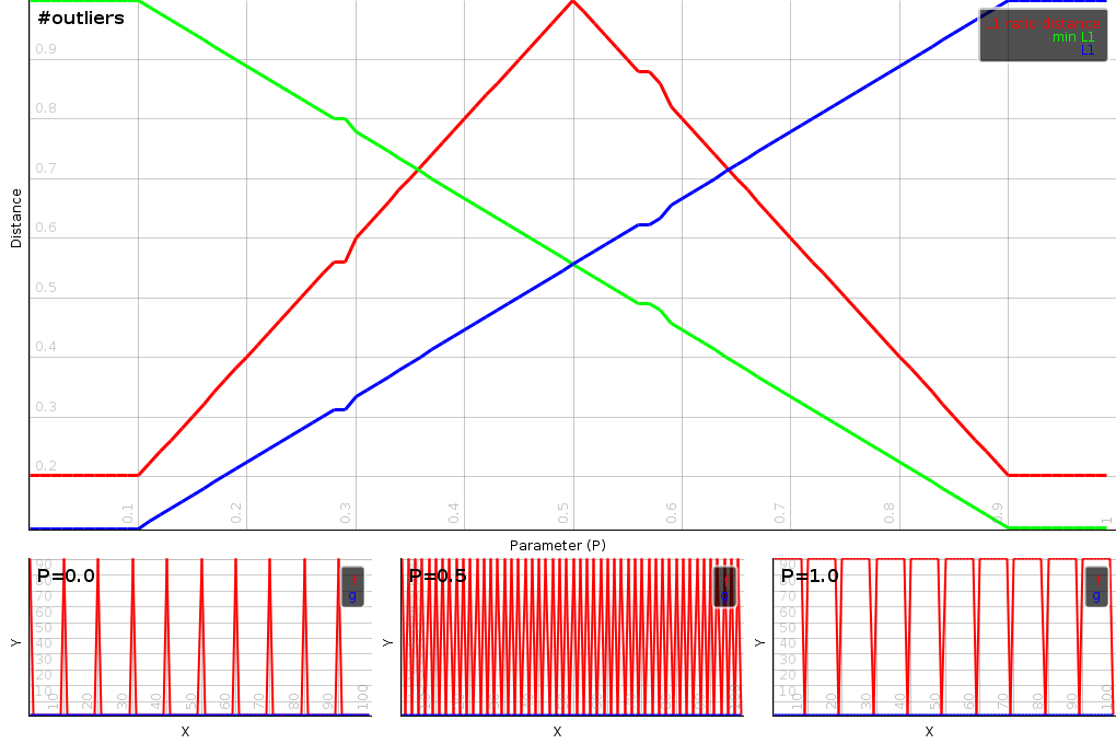
A gradual change from a small noise vector to a small noise vector with a large outlier. The L1 distance is linearly affected. The minimized L1 distance is less sensitive to the outlier, yet for small value it is. The minimized ratio-distance is completely oblivious to the outlier
|
The ratio distance is however not unsensitive to the number of outliers present. To demonstrate that we start out with a vector with 10 outliers. We gradually increase the number of outliers to 50% after which the number of outliers decreases again. The L1 distance is directly sensitive to the outliers. The minimal L1-distance is sensitive to the number of outliers in a weird inverted way. The minimal l1-ratio distance measures the number of outliers correctly. The distance will increase to 50% after which it decreases again.
|
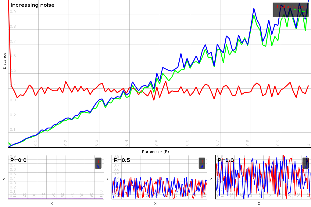
The minimal L1-ratio distance is unsesnsitive to noise. It will add an overall bias to the distance, but this bias will not depend on the actual level of the noise, which is a very weird feature indeed. To demonstrate that we gradually increase the level of uniform noise and plot the distances between the vectors. Both the L1 and minimal L1 distance react linearly. The minimal L1 ratio distance is pretty much a flat line.
|
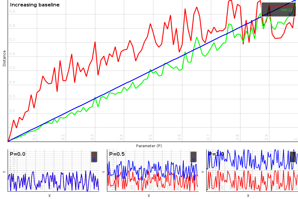
The minimal L1-ratio distance is sensitive to the bassline of the vectors. To demonstrate this we started out with a noise vector, which we then slowly shifted further apart. Practically, all three distances are sensitive to such a shift, the mijnimal L1- ratio distance is simply more sensitive. This is somethign that is desirable whgen working with audio vectors. Raising the energy level with a term is the same as adding a level of compression to the audio. Hence being sensitive to it is a good thing.
|
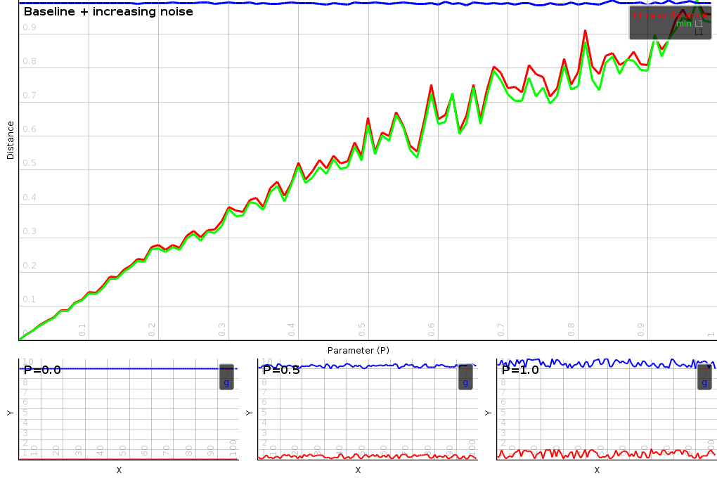
The unsensitivity to noise, yet the sensitivity to the bassline can further be explored by creating to noise vectors a certain distance away from each other. In this case we see that the minimal L1-ratio distance becomes sensitive to noise. The best way to describe this is: if there is a bassline present then the noise levels matter. If there is no bassline, then the noiselevels no longer matter.
|
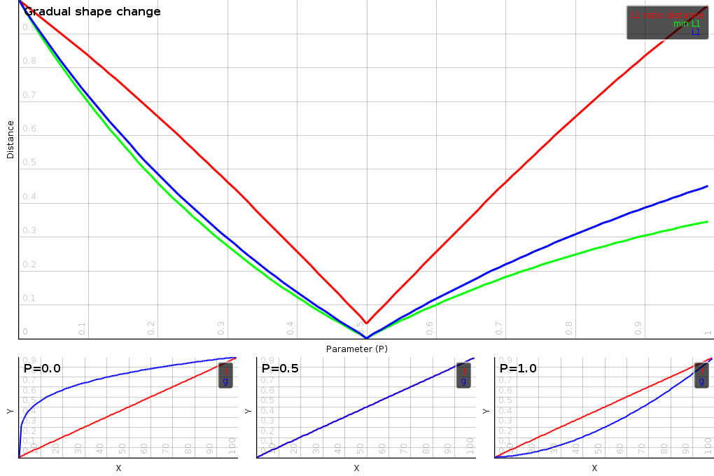
The gradual change of shape between vectors can also be tested. All three distances are sensitive to it. Yet the minimal L1-ratio distance seems to make the most coherent assessment. After all the difference in shape between a P value of 0 and 1 is pretty much the same. At P 0 the blue curve is x^0.25. At P 1 the blue curve is x^1.75. Both are a power 0.75 away from linearity.
Ratio distance between complex energy vectors
In previous section we described a method to compare energy levels, which can also be used on the energy levels of a spectrum. Yet, because a spectrum contains complex values, comparable bins could potentially cancel out if their phases were out of alignment. In that case, how should we compare them ?
One strategy could be to combine a ratio distance on the modus with an extra penalty for the difference between the angles. However, we found an easier solution by comparing the energy we have after subtraction, against the maximal energy we could have seen.
Instead of comparing x with y through division, we will compare
them as
 . This
value will be 0 when x and y are exactly the same (same modus and
argument). If the argument starts to diverge some rest signal will
remain, which will increase c. To map c back to something that
produces 1 when the signal is the same (so we can insert it in a
logarithm later), we will compare them through a bilinear
transform:
. This
value will be 0 when x and y are exactly the same (same modus and
argument). If the argument starts to diverge some rest signal will
remain, which will increase c. To map c back to something that
produces 1 when the signal is the same (so we can insert it in a
logarithm later), we will compare them through a bilinear
transform:
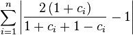
| Equation wopper: |  |
This value will be 1 when x and y are the same. When the arguments
of x and y are the same, then the outcome
of eq. wopper is either
 or
or
 .
.
Taking the logarithm of this equation and inserting it in the logistic function gives
| Equation complex-ratio-distance: |  |
| ||||
| The impact of phase on the terms of the distance. |
In L1 we get the follolwing
When the slope is 1 we have the following simplification
 | |  |
|  | |
|  | |
|  |
Which is the weirdest result. After all this technical work: determining a suitable comparator (c), a bilinear transform, taking its logarithm, inserting it into a logistic function, we find the sum of the c values back. Compare this with the original ratio distance and you'll see that only modus operators have been added in the denominator.
When the slope is not 1, it is easier to compute the c_{i} and the distance using equation complex-ratio-distance.
The function is almost always a smooth function, unless the phases of all positions are in alignment and we have a p=1, s=1 distance in use. That means that we can effectively use Newtons method to find a minimum.
Summary
The two most commonly used energy representations are acoustically wrong. The distance between RMS vectors increases when the volume of the two vectors increases and the distance between dB vectors is dominated by the most silent contributions of the signals.
Almost none of the most common normalization methods help us find the minimum distance when additive or multiplicative volume changes are allowed. The only one that works is subtracting the average from a dB vector when we use the L2-distance.
To minimize the L1-distance between dB vectors, one needs to
subtract the median of the difference from the terms in the distance
(section l1-add). For RMS vectors, the
L1-distance can be normalized by calculating the global minimum of a
convex curve as described in
section l1-plain. The L2 distance can be
minimized by setting to the value specified in
section l2-mult.
Afterwards we presented a method to compare the ratios between RMS vectors. We did this by dividing their energies and limiting the outcome through a logistic function. We presented a minimization approach for L1 and L2. Afterwards we explained how a distance between a complex energy representation can be created.
We did not yet discuss the application of weights in the distance functions, nor did we explain the qualitative difference between L1 and L2 optimization (try it, or Google 'm)
Finally, I would like to thank Nicklas Andersen for proofreading this document.
| http://werner.yellowcouch.org/ werner@yellowcouch.org |  |