| Home | Papers | Reports | Projects | Code Fragments | Dissertations | Presentations | Posters | Proposals | Lectures given | Course notes |
|
|
Fast Exponential EnvelopesWerner Van Belle1 - werner@yellowcouch.org, werner.van.belle@gmail.com Abstract : Computing ADSR curves is a task any synth has to deal with. In this article I present a method to compute exponential patches quickly and incrementally. Namely by multiplying the last envelopevalue with a constant multiplier (r) and then adding a constant delta (d) to it. This solution is used in the Audiotool Heisenberg synth to generate ADSR curves for pitch as well as amplitude.
Keywords:
ADSR Envelopes, Exponential Patches, Incremental offsetted exponential |
Table Of Contents
Recipe
The presented solution is based on exponential patches of which the linearity can be chosen as wanted.
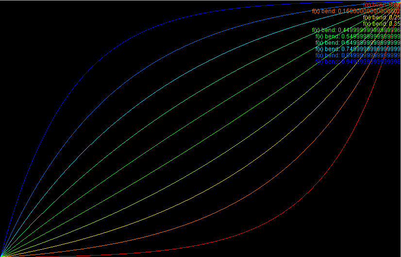 Illustrating the various curves that can be drawn.
|
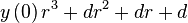
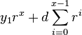
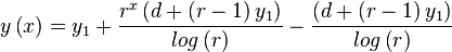
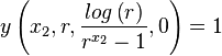
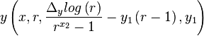
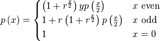
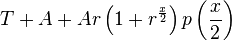
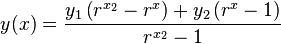
The following equation

| Equation main: | 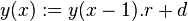 |
can be used to draw arbitrary exponential curves through three points

This can be done by choosing correct values for r and d, as follows:
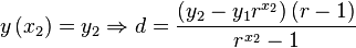
- Choose the width x2, start value y1, stop value y2 and the midpoint value

- Calculate
- Calculate
. - Set
 and then calculate
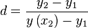
Computation of 
To calculate , given d, r, and y1 values:
- odd:=0
even := d
logr := log(r)
- while x>1
- if x is odd then
odd := odd + even
even := even * r - in all cases:
x := x >> 1
even := even * ( + 1)
+ 1)
- if x is odd then
- y := y1 + even + odd
The above algorithm can be computed in  .
.
Analytic Form 1
Equation main describes how
can be incrementally calculated. It
actually was created first because it is fast and because we assumed
that we could draw any exponential patch with it. Further study
provided than various analytic forms.
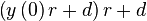
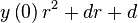
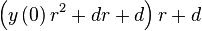
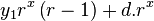
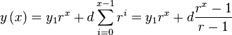
To determine a direct form of equation main, we set up the following series of dependencies, that then provides us with the resulting equation:
 |  |  |
 | |  |
 | |  |
|  | |
|  | |
 | |  |
|  | |
|  | |
 |
| Equation analytic1: | 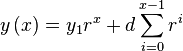 |
The direct form is thus equivalent to
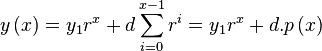
| Equation ypx: |  |
The section Series of Powers describes
how  can be
calculated. Section analytic form 4 provides the
most current revision of the algorithm.
can be
calculated. Section analytic form 4 provides the
most current revision of the algorithm.
Analytic Form 2
To obtain a second analytic form we can investigate the differential
of and see whether the integration is sensible.
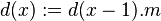
Differential of y(x)
To calculate the differential we subtract y(x) from y(x+1) and name the result d(x). d(x) will thus give us at each x position the value that should be added to the current y.
 | |  |
| |  |
 | |  |
| Equation diff: |  |
This function is an exponential, indicating that we could calculate y(x) slightly different, namely by calculating the differential in an incremental fashion and accumulating these values. Section Incremental based on differential focuses on an alternate method to compute y based on this insight. At the moment however, a differential that is an exponential begs to be integrated.
Integrating the Differential of y(x)
Integrating the equation of the differential gives a y-translated version of y(x), namely
| Equation integral: | 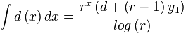 |
At x=0, a translated version of the integral should run through y1, which gives the following
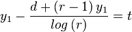
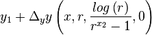
Thus, another analytic form is
| Equation analytical2: | 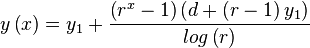 |
Equation analytical2 is a tricky beast to calculate because the ratio r can be 1, in which case log(r)=0, resulting in a division by 0. Secondly this equation is made using integration and differentiation which both assumed a continuous space. For integer values this will thus not work entirely correctly. See section Analytic form 4 for a better calculation.
Analytic form 3
In this section we study how we can offset and scale the curve. That will eventually allow us to write a normalized curve that goes from y1=0 to y2=1. That normalized curve can then be solved against r and d and subsequently scaled and translated back to its wanted position.
Because it is necessary below that we denote exactly which function we are talking about we will no longer write y(x), but rather y(x,r,d,i) in which x the point is where we want to know the value of the curve. r specifies the ratio multiplier. d specifies the delta added with each cycle and i specifies the initial condition. y(x,r,d,i) will be a non-normalized curve. The normalized curve will be called

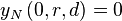
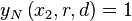
It will be normalized such that
Offsetting
We now aim to understand how offsetting a curve affects the values r and d. Or rather how we can, given a type of y-function (called f), modify r and d such that the new function g is shifted along the y axis.
| Equation wish: |  |
The above equation can be satisfied by simply ensuring that the shape of f and g are the same. (This is possible because the values at x=0 is for both curves already the same. Consequently we will only be looking at f' and g'.


If we now set  we obtain an expression for
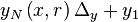
This result allows us to write the following
| Equation yshift: |  |
Scaling
To scale an exponential patch we merely need to multiply d with the required scaling factor m, as shown below

Scaling and Offsetting
Once we know $r$ for an unscaled, zero-offset function, we can first
scale it to reach  and the offset it to start at .
This is done as follows:
and the offset it to start at .
This is done as follows:
| Equation offsetandscale: |  |
A Normalized Curve
Given that we can scale and offset the curve any way we want, it is
time to create a normalized curve that goes from  over
over  to
to  .
.
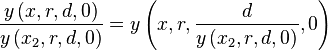
To start at position 0, it suffices to set the fourth argument to y to 0.
To scale the curve such that after x2 steps  is reached, it suffices to set d to the inverse of the value at
that position.
is reached, it suffices to set d to the inverse of the value at
that position.
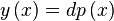
The calculation of>/p>
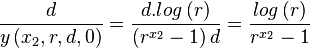
leads to
which thus means that
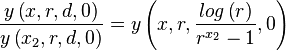
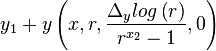
and that the equation for the unscaled curve is
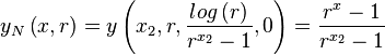
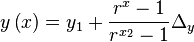
Which is an interesting result because the normalized curve depends only on r and no longer on d. It is also interesting because scaling and offsetting is something we can do after the facts, leading to the following third analytic form
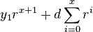
The fact that we have an equation for  and for the unscaled
equation makes it possible to write the analytic form of before as
a multiple of powers. Namely
and for the unscaled
equation makes it possible to write the analytic form of before as
a multiple of powers. Namely
Determining the multiplier
In this section we determine values for r such that the
resulting curve  goes through
the point
goes through
the point 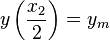 . This
means that the normalized curve should go through
.
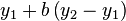
The y value of the last point will be called b. Given the
equation for the normalized curve we can write
. This
means that the normalized curve should go through
.
The y value of the last point will be called b. Given the
equation for the normalized curve we can write
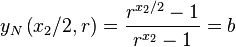
Defining  gives us
 | |  |
 | | |
 | |  |
 | | |
 | |  |
Given this value for r we can now scale the equation correctly and offset it
 | |  |
|  | |
|  |
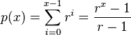
Computing the serie of powers
This section explains how to calculate p(x) and was created in absence of a sensible solution. See section analytic form 4 for a more up to date solution
Equation ypx poses a slight computational challenge since we potentially have to perform x steps to calculate p its value (A Horner scheme should not be considered because of that). Factorization of the polynomial in prime numbers could be a worthwhile attempt, but is unnecessary, because it is easier to realize that all coefficients of the polynomial are 1. This makes it possible to split the polynomial in two when we want.
 | |  |
|  | |
|  | |
|  |
When the polynomial is of uneven order we can work with the even part of of the polynomial and remember the remainder
 | |  |
|  | |
|  |
Combining these two branches gives (in which we assume that x/2 is performed as integer division).
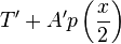
To create a non-recursive loop of the above we work with a term (which accumulates the 1's form the odd part) and an accumulator (which calculates the current value of $y\left(x\right)$). We write an equation of the form
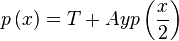
With start condition


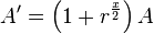
when x=0. When x is even we have

which shows how we calculated the new T' and A' to go into the next step

In the odd case we have
 | | 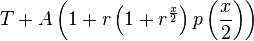 |
|  | |
|  |
In this case

This loop must finally be multiplied with d, as to obtain the correct value of y.
which leads to the two following insights regarding the odd and even cases.
 |  |  |
 |  |
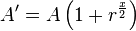
By integrating d into A for the initial case we effectively multiply A throughout the entire chain, leaving
 | |  |
 |  |
If we do the same for T (which starts of at 0), we see that
 |  | |
| |
Consequently. It suffices to start the calculation of y as a calculation of p and set the initial value of A to d.
A last improvement on the algorithm is that the term  ,
which can be rewritten as
,
which can be rewritten as
which has a constant  .
.
Analytic form 4
Thus
Determining d
Which means that, after some deductions
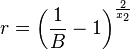
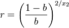
Determining r
To determine r we use the bend factor b (the relative point through which the curve should go at midpoint (x1+x2)/2.
 | |  |
| ||
 | |  |
Then assuming that

gives us the solution for the quadratic equation

the other solution is s=1. The end result is thus that
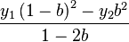
Plugging r and d into the equation eventually leads to the following expression
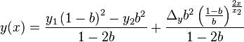
which itself can be written as
| |  |
 | |  |
 | |  |
 | |  |
Incremental calculation based on the differential
Because the differential of y (Eq. diff is an exponential curve, we could consider calculating the delta at each step, relying on an incremental scheme to calculate the exponential and then add that delta to the current running envelope.
To calculate an exponential increasing/decreasing  one merely
needs to decide on the multiplier for each step, which would then
result in the following:
one merely
needs to decide on the multiplier for each step, which would then
result in the following:


At each step we would perform the following
| Equation alternate: | 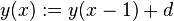 |
Below a breakdown of the differences in operation counts between equation main and and equation alternate.
| Method | Main | Alternate |
| Variable reads | 1 (y) | 2 (d, y) |
| Constant read | 2 (r, d) | 1 (m) |
| Variable writes | 1 (y) | 2 (d, y) |
| Multiplication | 1 (y.r) | 1 (d.m) |
| Additions | 1 (y.r + d) | 1 (y+d) |
The main difference between both is 1 variable write less, which in a very crude 'every operation is equally expensive' would mean that our presented methods is about 16% faster than the alternate.
Acknowledgments & History
The first verison of this document was written in April 2012. In may 2012 Anthony Liekens found an analytic solution for p(x), which resulted in an extension of this document (the fourth analytic variant).
Code
The code below is provided after someone kept on polling me on what was wrong with the recipe at the start of the article. Then I figured out that a numbner of offsets were wrong and that it would have been too much work to actually rectify them. Given that the recipe at the start of the document was also already outdated, I opted for providing working code directly. Enjoy it. If you use this code please refer to this article in your code as well as in your applications about box. Thank you.
/**
* To use this code incrementally, start with
*
* y = y1
*
* At each step set
*
* y = y * multiplier + delta
*
* After x2 steps, y will be y2. The curve will go through ym at halfwidth.
*
* @author Werner Van Belle (werner@yellowcouch.org)
*/
public double multiplier;
public double delta;
private double y1;
private double y2;
private double x2;
private double dy;
private double cstA;
private double cstD;
private double cstE;
private int branch = 0;
static final private double BEND_LINEAR_LOWER = 0.499999;
static final private double BEND_LINEAR_UPPER = 0.500001;
/**
* Curve will run through (0,y1), (x2/2,ym) and (x2,y2)
*/
public void setCoordinates(final double x2, final double y1, final double ym, final double y2)
{
if (y2 == y1)
setCoordinatesWithBend(x2, y1, 0.5, y1);
else
{
final double bend = ( ym - y1 ) / ( y2 - y1 );
assert(bend > 0 && bend < 1);
setCoordinatesWithBend(x2, y1, bend, y2);
}
}
public void setCoordinatesWithBend(double x2, double y1, double bend, double y2)
{
dy = y2 - y1;
this.y1 = y1;
this.x2 = x2;
this.y2 = y2;
if (bend>BEND_LINEAR_LOWER && bend<BEND_LINEAR_UPPER)
{
multiplier = 1;
delta = dy / x2;
branch=2;
}
else
{
final double onemb = 1 - bend;
final double onembs = onemb * onemb;
final double onem2b = 1- bend - bend;
final double bends = bend * bend;
final double s = onemb/bend;
multiplier = Math.pow(s,2/x2);
final double s2 = s * s;
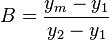
delta = ( y2 - y1 * s2 ) * ( multiplier - 1 ) / ( s2 - 1 );
cstA = ( y1 * onembs - y2 * bends ) / onem2b ;
double B = dy * bends / onem2b;
cstD = 2 * Math.log(s)/x2;
cstE = Math.log(Math.abs(B));
if (B<0) branch=1;
else branch=0;
}
}
/**
* Calculates y for a given x. X ranges from 0 to x2.
*
* @param x the position of which we want to know the y value
* @return
*/
public final double y(double x)
{
assert(x>=0);
if (branch == 0)
return cstA + Math.exp( cstD * x + cstE );
else if (branch == 1)
return cstA - Math.exp( cstD * x + cstE );
else
return y1 + x * dy / x2;
}
public double x(double y)
{
if (dy<0)
{
if (y>y1)
severe("dy<0 but y>y1");
}
else
{
if (y<y1)
severe("dy>0 but y<y1");
}
if ( branch == 0 )
return (Math.log( y - cstA) - cstE)/ cstD;
else if ( branch == 1)
return (Math.log( cstA - y ) - cstE)/ cstD;
else
// Use a linear approximation
return ( y - y1 ) * x2 / dy;
}
Summary
We presented a method to calculate an exponential patch quickly, using only 1 multiplication and 1 addition per sample. To make this possible, an algorithm was presented to calculate the required multiplier and delta, while at the same time providing a direct calculation of y(x).
Although, this is the essence of a fast ADSR envelope, it is clear that these patches need to be pieced together within a larger program, that will at appropriate times (when changing from Attack to Decay, or Sustain to Release) set new values for the multiplier and delta.
| http://werner.yellowcouch.org/ werner@yellowcouch.org |  |