| Home | Papers | Reports | Projects | Code Fragments | Dissertations | Presentations | Posters | Proposals | Lectures given | Course notes |
|
|
Bitslicing: Nearest Neighbors with <30% Data Access for 1000+ Dimensional Uniform SpacesWerner Van Belle1 - werner@yellowcouch.org, werner.van.belle@gmail.com Abstract : We describe a space partitioning scheme to store and retrieve high dimensional integer data (>1000 dimensions). The search structure is similar to hypertrees but retrieves the k nearest neighbors by accessing only ~30% of the search space. To make this possible, a breadth-first search culls away large areas of the space by using an incremental calculation of the minimal distance between each subspace and the point-of-interest.
Keywords:
k-NN, nearest neigbors, bitslicer technique, high dimensional data |
Table Of Contents
Introduction
We focus on the k nearest neighbor problem, which is the following: given a collection of N-dimensional points, return the k points that are closest to a point of interest. This type of querying can be useful for a DJ program that needs to retrieve songs with similar rhythmical patterns/composition properties or echo characteristics, to perform image searching or to study the structure of highly dimensional data before deciding how to get a grip on the dimensionality of the problem.
The k-nearest neighbors problem is fairly hard. Most techniques access >97% of the searchspace to produce a correct answer.
Why is multidimensional searching such a nightmare ?
Most people, that don't know the kNN problem, are often surprised to find that it such a hard problem. This is because it is easy to believe that space partitioning can solve almost all search problems. This is not the case. Nevertheless, explaining why partitioning does not work, is a completely different matter. I'll try to rephrase the problem a number of times.
The density argument - What could be so difficult on finding the closest neighbors. If I draw a collection of points on paper, I can simply draw a circle and figure out which elements are inside that circle. If I don't have sufficient elements, I can simply increase the radius to include more elements. The problem is that as soon as we go to higher dimensions the space becomes much less populated. For each point in the space, we will tend to have much more free space than we would have in lower dimensions. E.g: suppose we have 10000 points in a 2 dimensional plane in which the values on each axis can only be positive <=255, then we have a point densitiy of 0.15 points per pixel. (10000/65536). If we however store these 10000 points in a 4 dimensional plane, our densitiy became 2.3*10^-6 ! If we go to 6000++ dimensions our densitiy becomes so close to zero that simply increasing the radius will no longer cut it since at each step we have relatively more space to investiagate and fewer points.
Space versus Local argument - Another way of putting the same argument forward is to considers the volume of the unit sphere against the volume of the unit-cube. This relation sinks to zero as the number of dimensions increase. In other words: everything will be far away and the number of points that can be 'close' (inside the sphere) will statistically sink to zero.
The no partitioning argument - As with binary trees (1 Dimensional), KD-trees/quadtrees (2 dimensional), octtrees (3 dimensional), we might think that a space partitioning might make sense. The problem is that to cull away vast areas of the space we will need to partition the space along each of its dimensions, which means that we have around 2^N subspaces at each partitioning. Since the number of subspaces exceeds easily the number of points in it, it make no sense anymore to partition the space like that. Other partitioning can only deal with a fraction of the points.
Permutations - Looking only into 25 dimensions of a 6000 dimensional space is not sufficient to cull anything away from that space. After inspecting 25 dimensions we still only calculated a small fraction of the true distance , which leaves us around 6000-25 dimensions, to make up for how far or how close the point under investigation might appear. If we looked at 3000 dimensions and are as close as possible to a point that we want, then we still have another 3000 dimensions left to screw up our 'current best match' up. Or the other way around: if we have a point that is extremely far, if we only look at 3000 dimensions, then we still have another 3000 dimensions left to become nearly as close as we want to the required target.
Distances all become the same - Other people describe that classic distance measures are meaningless in high dimensional spaces. The argument goes that all points tend to be far from each other. In other words: the distances tend to become all more or less the same, with a low variance.
Intuitive understanding - All the above arguments deal with numbers, they do however not necessarily help you to understand the problem, so I'll go out on a limb here and explain it in more non scientific terms: you are a human on planet earth. Now, look into the sky with a telescope. Anything that is not earth tends to be extremely far away. Almost everything in the night sky is ridiculous far away. Nothing is truly close,If we would like to find the next 100 close objects in heaven (aside from the the ones in our solar system), we are faced with the same problem. How can we decide which part of the night-sky to investigate ? Remember that these are only 3 dimensions !
The above arguments led to a situation where some people in the field argue that distances in high dimensional spaces are meaningless. I disagree with that flawed line of reasoning. It is not because the problem is hard, that it should be classified as a meaningless problem, because 'the distances are so tricky'. It is a form of self delusion: we found an underlying 'deeper' (that is how we must call it then) cause for our problem, hence our problem must be flawed. This entire argument signals defeat.
State of the Art
P-trees decompose a n-dimensional space in 2n pyramidal subspaces. Each point in such a subspace is hashed based on its distance to the pyramid top. That hash together with the pyramid identification is then used to store the data in a standard linear search structure. The authors claim a relative data-access of about 10% (and according to them does not show any degradation at higher dimensions), but forget to mention that the datasize increases linearly with the number of pyramids they have, meaning that the relative page access to its own total size may well be 10%, but when plotting the relative page access compared against the size of the original dataset they would quickly find a number beyond 100% data-access. Furthermore they claim a K-nearest neighbor search is performed, while in reality they can only perform range queries. Some follow-up papers also noticed that P-tree require an adaptation to work on general purpose queries. [1, 2]
The X-tree, another invention by the same group has the more expected data access times. Figure 2 in [1] illustrates a relative page access of 100% beyond 10 dimensions. The original paper does not report anything beyond 16 dimensions.
Another strategy creates geometrical objects in the solution space (Voronoi cells) and uses that to index the space. Each cell consists of all potential query points which have the corresponding data point as a nearest neighbor. The cells therefore correspond to the d-dimensional Voronoi cells. Determining the nearest neighbor of a query point now becomes equivalent to determining the Voronoi cell in which the query point is located [3]. Although an interesting approach, the paper does not provide numbers on how much of the search space was accessed. Page counts are listed but how many pages there were is unclear. Nevertheless, the plots never exceed 16 dimensions.
[4] describes a strategy to use space-filling curves to index the search space, but does not go beyond 256 dimensions. It also allows points to go missing in action. In their experiment 90% of the correct resultset was returned.
Hashing techniques have also been considered. One is 'iDistance', which uses a number of random points as center. Towards these centers the distances are calculated. Each query is translated to a number of range queries on multiple indices [5]. Another one are local sensitive hashes [6]. However experiments in BpmDj showed that the hash functions have a number of more sensitive areas in the searchspace and the results always felt biased towards certain ares.
The Bitslicer Technique
Below we present the bitslicer technique, which reduces the data access to about 30-40%. We will assume that dimensionality reduction techniques are not applicable because our problem is truly high dimensional. That means that each of the dimensions is fully independent of all other dimensions.
To test our algorithm we used a number of Monte-Carlo simulations with N-dimensional uniformly distributed random points. This being the hardest problem, one can always add problem specific improvements such as eigenvector analysis, dimensional reorganization, feature vector extraction and other dimensionality reduction techniques.
When we report relative data accesses we divided the number of bits (pages) accessed to create a complete resultset by the numbers of bits/pages it would take to store all points sequentially on disk.
Space and Metric
The points are N dimensional.
The elements of each point (p1, p2, ... pn) are positive integers up to a certain maximum value, defined by its bit depth. E.g: p_i can have values from 0 to 255 (8 bits) or from 0 to 65535 (16 bits).
Our solution is further firmly tied into the metric defined on this space, namely the L1 distance
Partitioning
The search structure is a tree in which each node represents a square (cubic/ hyper-cubic) area of the searchspace. Every node contains a list of non-empty children (also nodes). The children represent corner subspaces of their parent. For instance in a 2 dimensional space, a square can be divided in 4 subspaces: (top-left, top-right, bottom-left and bottom-right). In 8 dimensions, the subspaces are front-top-left, front-top-right, front-bottom-left, front-bottom-right, back-top-left, back-top-right, back-bottom-left and back-bottom-right. For higher dimensions this division continues and results in a potential of 2^N children at each node. Each child can be uniquely identified using N bits. E.g: when bit 3 is 'on' then we are dealing with children at the 'large-valued' end of the third dimension.
Storing a point in this structure is done recursively. At each node it is decided which of the children will contain the point. If there was no appropriate child yet, one is created. The interesting thing now is that a bitslice of the point-to-be stored can be used as an address to find the correct child. At tree depth x, the N bits (one for each dimension) at bit number bitdepth-x of the point-to-be-stored can be concatenated and used as an address to identify the correct child. E.g: in a 3 dimensional search structure with 6-bit values, only 8 addresses are necessary to uniquely identify all of a node its children (000, 001, 010, 011, 100, 101, 110, 111). If we want to store a point in this tree, at the root we merely need to look at bit 5 of each of the 3 coordinate-values. These 3 bits correspond to the corner space to which the point belongs. When then storing the point into that child, bit 4 will defines which grand-child is appropriate. This process continues until no bits are left.
When the correct node is reached in the tree, one could store the point. That is however not strictly necessary because the path from the root to the target node fully defines the point that would be stored there. So when no meta-information is associated with the point, it is unnecessary to have a direct representation of the point.
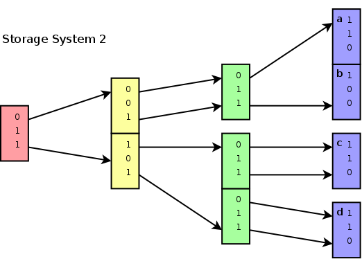
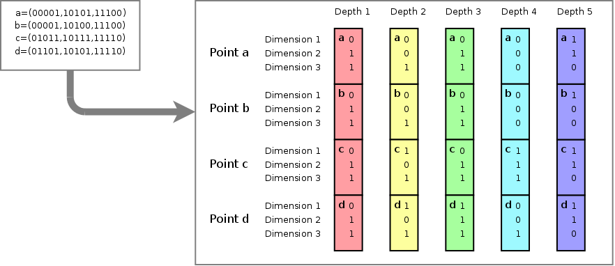 4 points {a,b,c and d}, each
having 3 dimensions and a bitdepth of 5. The image shows how the bits
for each value at each dimension specify the subspace to which a
particular point belongs. For instance, points a,b,c and d all belong
to subspace 001 at depth 1. At depth 2, point a and b belong to
subspace 001 (of the parent space 001), while point c and d belong to
subspace 101 (of the parent space 001). Point d for instance is fully
described by its subspace 110 (purple) of parent space 001 (cyan), of
parent space 111 (green) of parent space 101 (yellow) of parent space
011 (red).
4 points {a,b,c and d}, each
having 3 dimensions and a bitdepth of 5. The image shows how the bits
for each value at each dimension specify the subspace to which a
particular point belongs. For instance, points a,b,c and d all belong
to subspace 001 at depth 1. At depth 2, point a and b belong to
subspace 001 (of the parent space 001), while point c and d belong to
subspace 101 (of the parent space 001). Point d for instance is fully
described by its subspace 110 (purple) of parent space 001 (cyan), of
parent space 111 (green) of parent space 101 (yellow) of parent space
011 (red).
|
The logical tree structure must be somehow serialized to disk. The most straightforward approach is to sequence each of the different bitdepths. Thereby we first store all most significant bits of all points, after which the lesser significant bits are stored, until the least significant bits of all points are stored.
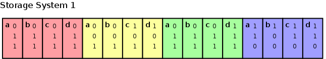 Storing the subspace addresses as
a flat structure
Storing the subspace addresses as
a flat structure
|
There are valuable improvements that can be made to both the representation as well as the storage-order. At the moment however, such a flat structure suffices to explain the working of the algorithm.
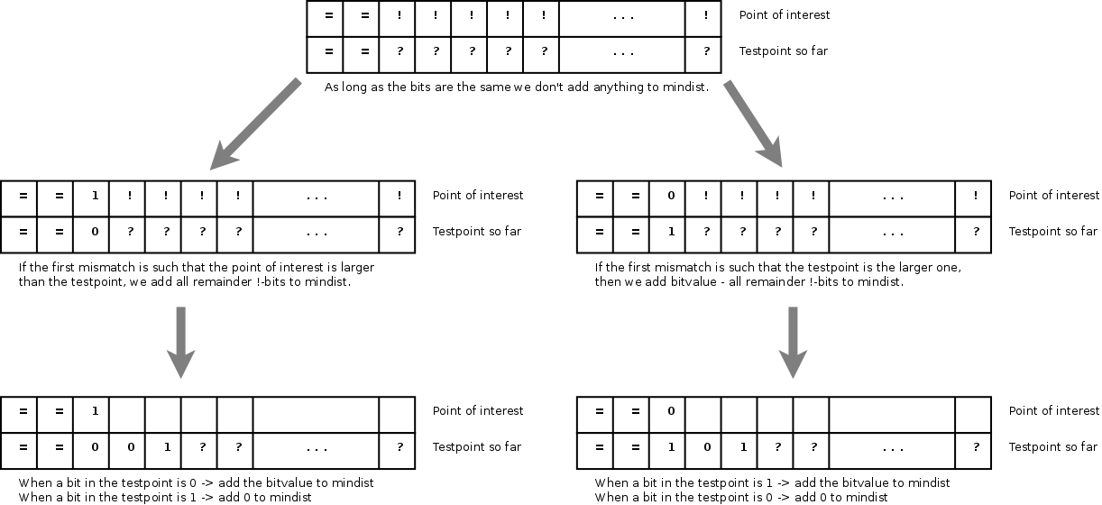
Culling: incremental absolute difference
To efficiently search for nearest neighbors, it would be nice if the algorithm could cull away subspaces, preferably at an early stage. To do so, we must be able to decide for each node what the smallest distance from any point underneath that node to the point-of-interest could be. As soon as the minimal distance of such a branch becomes larger than the best distance so far, we can reject that entire branch.
The problem is of course that the branches reveal themselves incrementally. At depth d, we simply don't know exactly which points are stored underneath. Each time we go one level deeper, we get a little bit more information on what points are stored. The point-of-interest on the other hand is fully known. In summary, we are looking for
- an algorithm that will tell us the minimal distance of any point in a particular branch towards the point-of interest
- the point-of-interest is fully known, but the bits of the stored points reveal themselves slowly and costly
- the algorithm should be an incrementally increasing function. If it weren't increasing we could never cull away a subspace because it could be recovered at a deeper stage, where the minimal distance could lower again.
That means that we should create an algorithm that can incrementally calculate the absolute difference, starting from the most significant bit to the least significant bit. This algorithm should only add positive values to the 'distance-so-far'
 Incremental calculation of the
absolute difference, starting at the most significant bit.
Incremental calculation of the
absolute difference, starting at the most significant bit.
|
An incremental absolute difference can be calculated by comparing the current most significant bits of the point of interest and the subspace address. As long as the bits are the same, the minimum distance from the point of interest to the subspace is 0. However, as soon the bits differ we know that the test point does not belong to the subspace identified by the child's' address. In that case we can directly add all remaining bits of the point-of-interest to the mindist and remember whether the point-of-interest or the subspace address was the largest. All following bits of the subspaces will then be properly added to the mindist. Below is a demo-implementation
/* create a point of interested and a testpoint */
int bits = 24;
int poi = random() % (1<<bits);
int test = random() % (1<<bits);

/* remembers whether we known which point is larger, and if we know it, whether the test point (the subspace) is the largest */
bool larger_known = false;
bool test_larger = false;

/* the accumulated distance */
unsigned long distsofar=0;

/* run from most signifanct to least significant */
for(int b = bits-1 ; b >=0 ; b--)
  {
    unsigned int bit_value = 1 << b;
    bool test_bit = bit_value & test;
    if (larger_known)
      {
	if (test_larger)
	  {
	    if (test_bit)
	      distsofar+=bit_value;
	  }
	else
	  {
	    if (!test_bit)
	      distsofar+=bit_value;
	  }
      }
    else
      {
	bool poi_bit = poi & bit_value;
	if (poi_bit != test_bit)
	  {
	    larger_known = true;
	    unsigned int masked_poi_value = poi_value & ( bit_value - 1 );
	    if (poi_bit)
	      {
		test_larger = false;
		distsofar += 1 + masked_poi_value;
	      }
	    else
	      {
		test_larger = true;
		distsofar += bit_value - masked_poi_value;
	      }
	  }
      }
  }
Searching
The above incremental distance calculation can be used to linearly search for nearest neighbors. Iterating over All bits, all points, all dimensions (in that order), the distance to the point-of-interest is calculated and added to a resultset, sorted according to distance. If the result queue contains more elements than wanted, it is shortened and we start working with a 'distance-should-be-smaller-than' value (which is the maximum distance present in the resultset + (2^remaining_bits)-1. Each time that we incrementally calculate the distance from the point-of-interest to the point-being-tested, we can break off as soon as distance-so-far>=distance-should-be-smaller-than.
Below an overview of the algorithm
- Place references to all points in the database in the resultset
- From the most significant bit to the least significant bit
- Iterate over all points< and update the minimum distance to the point of interest
- Find the k loweste minimum distance and add 2^remaining_bits-1. This value is the cutoff value
- Remove all elements from the resultset that have a minimum_distance larger than the cutoff value
Monte-Carlo Simulation
Bitaccesses
The data accesses in the above algorithm can be calculated using a Monte-Carlo simulation. Thereby, dimensionality, bitdepth, searchpct (how many % of the points we want to retrieve) and load (how many points are stored) are relevant.
Effect of Dimensionality
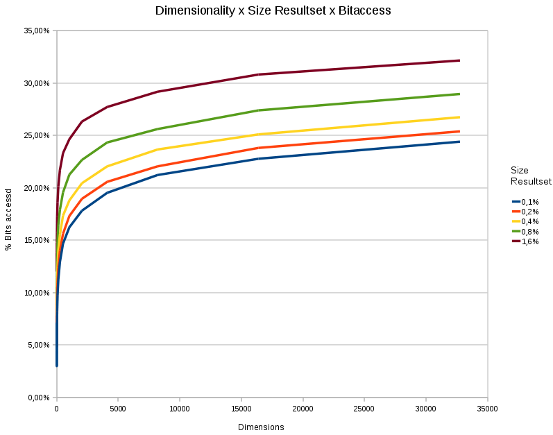 A chart showing the %
bitaccess under different dimensions and different resultsetsizes. The
total number of points in each test was 65536. The bitdepth was 31
bits.
A chart showing the %
bitaccess under different dimensions and different resultsetsizes. The
total number of points in each test was 65536. The bitdepth was 31
bits.
|
- The data access depends logarithmically on the dimensionality.
- The data access responds linearly to the wanted size of the resultset.
Effect of Loading & Size of the Resultset
| ||||
| Horzintal the # of points stored in the space is set out. Vertically, how many % of the searchspace we access. Each curve is of different dimensionality. All values are 30 bits. The average size of each resultset was percentually the same. |
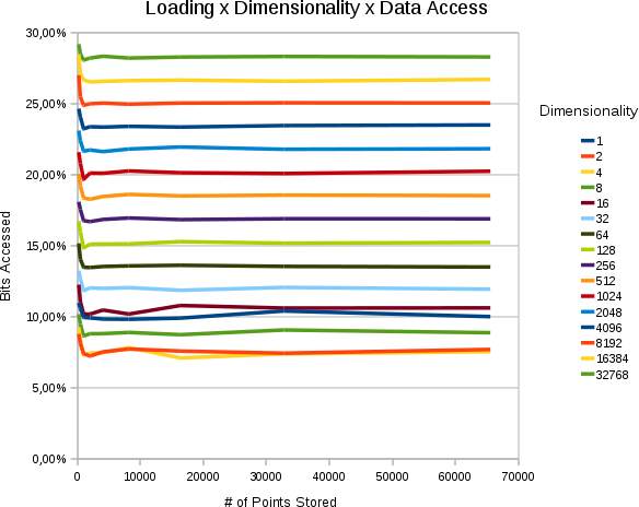
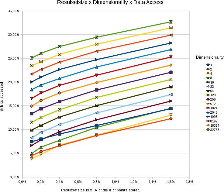
- The % of the searchspace accessed is a constant that depends on the percentual size of the resultset and the dimensionality
- The % of the searchspace accessed does not depend on the numbers of points stored.
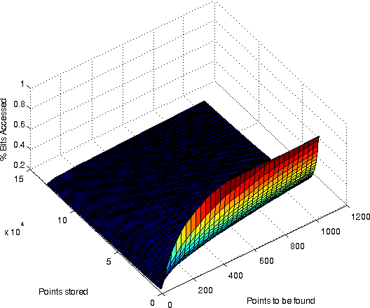 A surface plot showing the % bitaccess for various combinations of resultsitsize and # of points stored. Dimensionality was 32768. Bits/value: 31
|
Effect of Bitdepth
When incrementally calculating the nearest neighbors, using a lower limit on the current search result, there are two aspects that determine whether a point at a certain bitdepth is truncated.
 How many bits did we see
before a decission could be made. Horizontally, the number of points
seen so far is set out. Vertically, the number of bits we looked at to
come to a decission. In this case a 32768 dimensional sapce was
searched with 31 bits/value. The resultsetsize was 262 points.
How many bits did we see
before a decission could be made. Horizontally, the number of points
seen so far is set out. Vertically, the number of bits we looked at to
come to a decission. In this case a 32768 dimensional sapce was
searched with 31 bits/value. The resultsetsize was 262 points.
|
- sometimes we encounter a point that belongs in the set. In that case, there will be no truncation at all and all bits will be investigated. As the resultset narrows down, the chance that a certain new point belongs to the resultset shrinks. This behaves more or less as a poison distribution.
- secondly, if the point does not belong to the resultset, the computation is truncated at a certain bitdepth. This we investigate below:
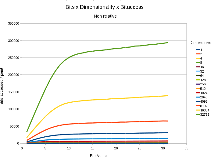
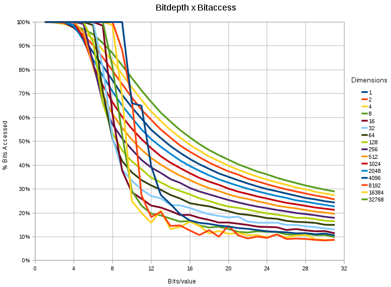 A chart showing the %
bitaccess under different dimensions and different bitdepth/value. In
all cases, the space contained 65536 points, and only 0.8% (524 point)
nearest neighbors had to be retrieved.
A chart showing the %
bitaccess under different dimensions and different bitdepth/value. In
all cases, the space contained 65536 points, and only 0.8% (524 point)
nearest neighbors had to be retrieved.
|
- The more bits we have the less relevant the 'lesser significant' bits become. Although apparently a tautology, it makes it possible to reduce the data access in a nearest neighbor problem substantially.
- When storing 16 bit values, the data access can be reduced to 50 % (for 32768 dimensional spaces), and even <30% for <256 dimensional spaces.
- When storing 32 bit values, the data access can be reduced to 30 % (for 32768 dimensional spaces), and even <20% for <256 dimensional spaces.
- When storing 8 bit values, there is little to be gained
- The effect is 'sudden' for lower dimensions (< 1024) and a relatively steep drop occurs between the 6th and 12th bit.
The presence of the threshold with respect to the bits/value is an interesting phenomenon
CDF: how often is bit x accessed ?
To study this phenomenon further it is useful to have a cumulative distribution that tells us how many % of the searches is stopped (or let through) at each bit.
Bitnumber versus truncation %
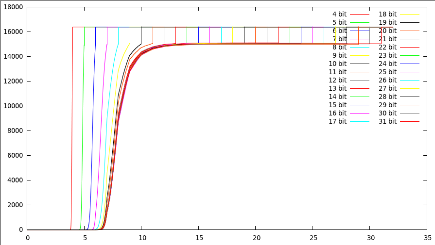 The cummulative distribution that
counts how many points were stopped after investigating x bits (bits
are set out horizontally, number of points stopped up to that bit are
set vertically). The space was 32768 dimensional, with a total of
16384 points. Each curve shows a different bits/value experiment. Each
curve start at 0 (no points were rejected yet), goes to a certain
threshold (bits 5...12), where it increases (at this bitdepth we start
to reject more and more points), after which it plateaus (it no longer
matter what we see now), to finally jump to the maximumvalue at its
maximumbitdepth. The margin at the top is normal, since after all, we
still need to look at all bits in about 30% of the cases.
The cummulative distribution that
counts how many points were stopped after investigating x bits (bits
are set out horizontally, number of points stopped up to that bit are
set vertically). The space was 32768 dimensional, with a total of
16384 points. Each curve shows a different bits/value experiment. Each
curve start at 0 (no points were rejected yet), goes to a certain
threshold (bits 5...12), where it increases (at this bitdepth we start
to reject more and more points), after which it plateaus (it no longer
matter what we see now), to finally jump to the maximumvalue at its
maximumbitdepth. The margin at the top is normal, since after all, we
still need to look at all bits in about 30% of the cases.
|
The first interesting thing to notice is that the threshold at which point we start deciding whether a point is still a potential result or not, depends little on the number of bits we have in the searchspace. In the above picture we have been searching a 32768 dimensional space, with 16384 points in it. Initially the points had only 4 bits, which we incrementally increased with each new experiment. The 26 shown curves illustrate that, if we have few bits, we need to look at all bits to decide whether the point does not belongs to the resultset. If we add bits to the values, we find that our threshold lays between bit 8 and 9. That means that those bits are the most relevant to decide whether a point is still a candidate for the resultset. Beyond bit 12 it simply no longer matters. Whether we have 12 bits or 32 is simply more comparisons, but will not add any value to the nearest neighbor problem. There are of course a number of interesting conclusions from this
- Having more than 12 bits is unnecessary in uniform 32768 dimensional spaces. (Now that is an interesting results, something that I was not expecting)
- Up to bit 8, we can't really decide anything, and we need to look at each individual bit.
Dimension & Bitnumber versus truncation %
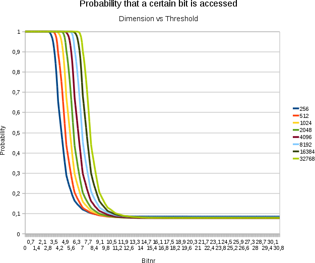 A plot demonstrating the
effect of increasing the dimensionality on the threshold. Horizontally
the bitnumbers are set out. Vertically the probability that a specific
bit at that position is accessed. Each test involved 16384 points with
31 bits/value
A plot demonstrating the
effect of increasing the dimensionality on the threshold. Horizontally
the bitnumbers are set out. Vertically the probability that a specific
bit at that position is accessed. Each test involved 16384 points with
31 bits/value
|
- The above graph illustrates how the threshold depends logarithmically on the dimensionality of the space, which is certainly an interesting result. Adding extra dimensions becomes less expensive the more we already had.
Page accesses
In the previous section I discussed the average number of bits we must access to find the nearest neighbors to a specific point. Of course, each bit access involves often a page access (either in memory, beyond the cache or on disk). Therefore it is somewhat important to have a look at the page accesses as well. Somewhat, because if pages are sufficiently large, many algorithms that involve random accesses can be crippled. Therefore, if this algorithm is to be used in real life one must consider architectures without overly large page sizes.
To test the performance of our algorithm on page-accesses, we've set up a Monte-Carlo simulation in which we laid out each points as a series of bits/dimension until a number of full pages have been filled. The remaining bits are aggregated and placed in a 'restblock'. Below an example of the layout we used to perform the simulation'
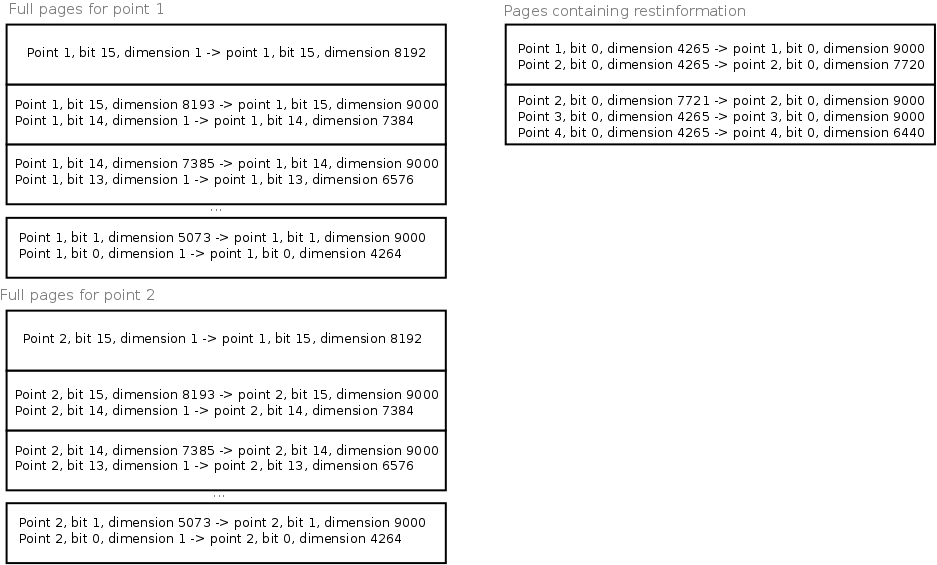 Pagelayout for points in a
9000 dimensional space with 16 bits / value. For each point we lay out
a number of full pages. The pagesize is 1024 bytes
Pagelayout for points in a
9000 dimensional space with 16 bits / value. For each point we lay out
a number of full pages. The pagesize is 1024 bytes
|
If we have a 9000 dimensional space with 16 bits/value, then we have in total 144000bits / point. With a pagesize of 1024 bytes (8192 bits/page), we need 17 full pages / point. These full pages are stored as they are. (See figure, part 'full pages for point 1' and 'full pages for point 2'). The remaining bits/point are stored sequentially in a set of 'rest'pages. With 4736 restbits/point, we can approximately store 1.7 point/restpage. (See the right part 'restpage' in the above figure').
One of the questions now is whether we store the most or least significant bits in the restpages (thus whether the bits numbered 0/15 are the most/least significant bits or vice versa). If we store the least significant bit in the restpages, we will create pages that we access seldom (because only 30% of the searches go that deep). The full pages will then contain more significant bits and thus each point access will be clearly delimited to one page, which appears good at first sight.
One could however also argue the other way around and place the lesser significant bits in their own pages. The reasoning to do that could be that we will, regardless of how 'more significant' the bit is, access it anyway, and therefore it would be better to allow the significant bits to be spread over multiple pages (we will access all of them anyway, so it doesn't matter). The lesser significant bits on the other hand are seldomly accessed and with a 10-30% change of accessing the lower bits it is better to keep that victory (not access that page) than to share it with another set of lesser bits that might be accessed in 30% of the tries as well.
Dimensions: 20480
Bits/value: 32
Pagesize: 1024
Searchresultsize: 32

Points  %Access
512     0.44543   0.454028  0.450293
1024    0.374724  0.384131  0.380005
1536    0.344043  0.353735  0.349512
2048    0.328733  0.338452  0.334283
2560    0.316139  0.325947  0.321802
A small experiment showed that the latter reasoning was sound. Below we tested a 20480 dimensional space with 32 bits/value and a pagesize of 1024 bytes. The three values printed are bitaccess/pageaccess with the least significant bits in restpages/pageaccesses with the most significant bits in the restpages.
The above strategy provides us with the largest gain when the number of restbits per point is half a page large. Nevertheless, the two presented approaches are two extremes. Other bit/page layouts are possible as well. To be able to calculate the gain of sharing bits or keeping them along it is useful to obtain the probability distribution that a certain bit will be accessed at a certain depth. Based on that we can create a page layout that, shares as many 'highly probably accessed bits' per page as possible (that is: this type of pages contain as many points as possible) while grouping together together the lesser accessed bits for each point into a single page. How this is done exactly depends on the type of distribution we are dealing with, and what the probability is that a specific bit will be accessed.
In general the question is whether we join in one page multiple bits of the same point or multiple points, but the same bit. As is already apparent, joining multiple bits of the same point is useful if the bits in question are seldomly accessed. On the other hand, if the bits are almost certainly accessed it makes more sense to place multiple points per page. What should happen at the transition area is somewhat unclear, it is however possible to write a program that will create an optimal page layout for the problem at hand
long bits=31;
long dimensions=128;
int points=10000;
long page_size_bytes = 1024;
double searchpct = 0.01;
float* prob_bit_access;  // Is a linear array to be addressed as bit x dimensions + dimension

long page_size_bits = page_size_bytes * 8;

struct BitAggregate
{
  int start;
  int length;
  float rel_page_access;
  BitAggregate(int st, int l)
  {
    start=st;
    length=l;
    rel_page_access=INFINITY;
  }
  float relative_page_access()
  {
    if (isinf(rel_page_access))
      rel_page_access=calculate_relative_page_access();
    return rel_page_access;
  }

  float calculate_relative_page_access()
  {
    // how many bits do we need to see to reach a full apge boundary ?
    long scan_length_bits=lcm(page_size_bits,length);
    long pages=scan_length_bits/page_size_bits;
    double relative_page_access = 0;
    for(int page = 0 ; page<pages;page++)
      {
	long start_bit=page*page_size_bits;
	long stop_bit=start_bit+page_size_bits;
	long current_point=-1;
	double prob_that_page_is_not_accessed=1;
	for(int bit=start_bit;bit<stop_bit; bit++)
	  {
	    long point=bit/length;
	    if (point==current_point) continue;
	    current_point=point;
	    long bit_in_point=bit%length;
	    assert(start+bit_in_point<=bits*dimensions);
	    double prob_that_bit_is_not_accessed=1.-prob_bit_access[start+bit_in_point];
	    prob_that_page_is_not_accessed*=prob_that_bit_is_not_accessed;
	  }
	double prob_that_page_is_accessed=1-prob_that_page_is_not_accessed;
	relative_page_access+=prob_that_page_is_accessed;
      }
    return relative_page_access/pages;
  }
};

typedef boost::shared_ptr<BitAggregate> Ba;

double layout_page_access(vector<Ba>* aggregates)
{
  double total=0;
  double prob_sum=0;
  for(int i = 0 ; i < aggregates->size(); i++)
    {
      Ba aggregate=(*aggregates)[i];
      double weight=aggregate->length;
      total+=weight;
      prob_sum+=aggregate->relative_page_access()*weight;
    };
  assert(total==bits*dimensions);
  return prob_sum/total;
}

void create_best_layout()
{
  vector<Ba> *aggregate=new vector<Ba>();
  vector<Ba> *new_aggregate=new vector<Ba>();
  int step=dimensions;
  for(int i = 0; i < bits*dimensions;i+=step)
    {
      Ba ba=Ba(new BitAggregate(i,step));
      new_aggregate->push_back(ba);
    }
  for(int i = new_aggregate->size()-1; i>=0; i--)
    aggregate->push_back((*new_aggregate)[i]);

  double old_page_access=1;
  for(int current_merging_point=0;current_merging_point<aggregate->size()-1; )
    {
      new_aggregate->clear();
      for(int i = 0 ; i < current_merging_point; i++)
	new_aggregate->push_back((*aggregate)[i]);
      Ba toextend1=(*aggregate)[current_merging_point];
      Ba toextend2=(*aggregate)[current_merging_point+1];
      if (toextend2->start==0) break;

      Ba extended=Ba(new BitAggregate(toextend2->start,toextend1->length+toextend2->length));
      new_aggregate->push_back(extended);

      for(int i = current_merging_point+2 ; i < aggregate->size(); i++)
	{
	  Ba a=(*aggregate)[i];
	  new_aggregate->push_back(a);
	}
      int s=new_aggregate->size();
      double new_page_access=layout_page_access(new_aggregate);
      cout << "At merging point " << current_merging_point << " layout: " << new_page_access;
      if (new_page_access<=old_page_access)
	{
	  cout << " merged bit " << (toextend2->start/dimensions) << " and " << (toextend1->start/dimensions) << ".\n";
	  old_page_access=new_page_access;
	  vector<Ba>* tmp=aggregate;
	  aggregate=new_aggregate;
	  new_aggregate=tmp;
	}
      else
	{
	  cout << " advance.\n";
	  current_merging_point++;
	}
    }
  cout << "Aggregate Size " << aggregate->size() << "\n";
}
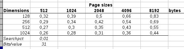 A sampling of various
combinations of pagesize versus dimensions and their respective
relative data accesses
A sampling of various
combinations of pagesize versus dimensions and their respective
relative data accesses
|
Non relative effects
Above we provided results in percentages (resultset was x % of the number of points stored, y % of the data store was accessed). It is nevertheless fairly useful to have a look at the absolute numbers. After all, it might be that we only access 30%, but if we have 32 bits instead of 16, we also doubled the size of the dataset.
| ||||
| A chart showing the relation between dimensionality, stored points, size of the wanted resultset and the average numbers of bits accessed per point. The space contained 65536 points, wit a 31bit/value depth. |
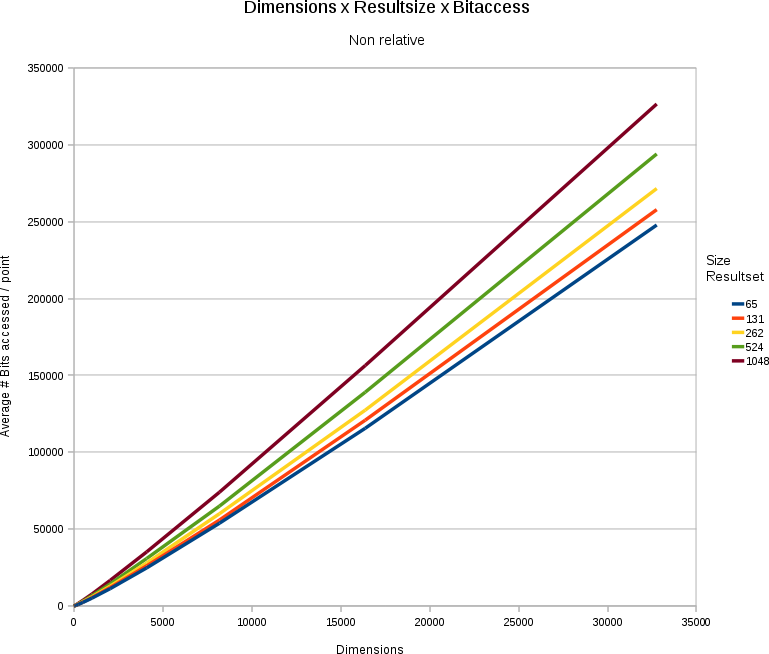
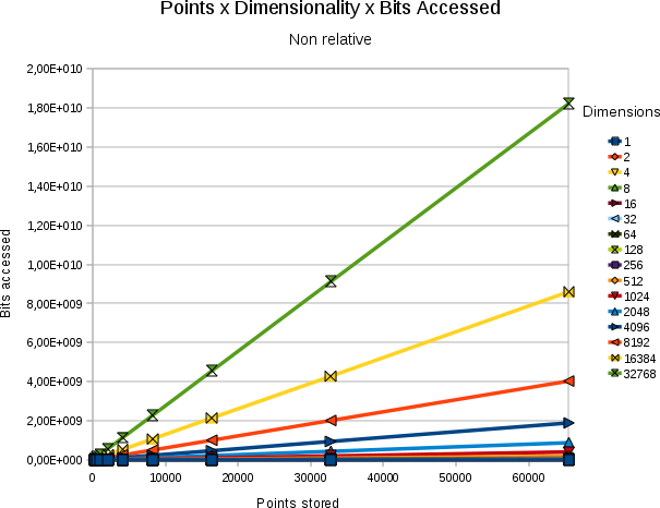
In general the problem remains linear. Although we only need to access between 20 and 30% of the searchspace, we still are talking about a solution that is linear towards
- the number of points stored (more points = more data access). For instance, in a 32768 dimensional space, with 30 bits/value, and a resultset-size that is a fixed % of the total number of points, we must access around 33.28 kB extra per search per point we add. (which is not bad, given that the point we added itself is 120 kB of data).
- the number of dimensions/point (more dimensions = more data access). For instance, if we have 65536 points in the store, with 31 bits/value. Each addition of an extra dimension will incur a data storage cost of 248 kilobytes. When searching the data however we only need to access 83.07 kilobytes extra.
- the number of results wanted (more results = more data access). For instance, if we have 31 bits/value in a 32768 dimensional space containing 65536 points, then for each extra point we want in the resultset we must access 495 kilobytes extra (in a space that is in total 7.75 gigabytes)
| ||||
| Absolute # of bits accessed for a variety of combinations of resultsetsize and point stored. In all cases the dimensionality was 32768 and bits/value 31 |
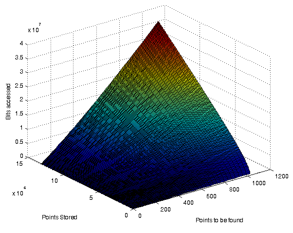
The relation between the absolute number of bits searched and the size of the resultset against the number of points stored is shown in the above figure.
If we set out the absolute numbers of bits searched given a certain bitdepth, we find the following plot.
 A chart showing the
absolute number of bitaccesses under different dimensions and
different bitdepth/value. In all cases, the space contained 65536
points, and only 0.8% (524 points) nearest neighbors had to be
retrieved.
A chart showing the
absolute number of bitaccesses under different dimensions and
different bitdepth/value. In all cases, the space contained 65536
points, and only 0.8% (524 points) nearest neighbors had to be
retrieved.
|
- If we use more bits/value, we must search more data.
- Up to a certain threshold, each extra bit/value costs its full amount.
- After the threshold (which is at bit ~12) each new extra bit starts to cost less.
Conclusions
We presented a k-nearest neighbors algorithm that brings down previous relative data-access rates from ~97% to ~30%. The algorithm reorganizes all bits within a point such that more significant bits are tested before lesser significant bits. To search this space an incremental absolute difference was created.
|
|
When only looking at bit-accesses we found results as pictured above. When dealing with hardware that can only access data in whole pages, an algorithm was presented to lay out the bits across pages, such that similar access rates can be kept for larger dimensional spaces.
Some interesting observations:
- there is an optimal number of bits that balances the resolution of the points against the amount of data to be looked upon during searching. It is not always advantageous to work with high resolution integers.
- There exists a threshold-bit at which the decision to throw out or keep a point is made or not. This transition bit is 3+log2(dimensions)/2.
Aside from being a nice theoretical realization, this algorithm is currently fairly expensive to implement on standard hardware. There are two grounds for this: 1- standard processors are not made to deal with individual bits. 2- for spaces that are high dimensional but for which the storage needs per point fall far below the pagesize (e.g: 64 dimensional spaces), the algorithm performs poorly. This is however related to the hardware. With new disks that by default use sector sizes of 16384 bytes (Western Digital produces really crap disks), most algorithms will start to feel an impact anyway. That does however not change the fact that this is the first algorithm to provide such low relative data-accesses.
Future Work
The presented Monte-Carlo simulations are interesting because they show a number of unexpected results. I tried to perform the statistics in a rigorous fashion but eventually, some parts of the statistics didn't have an analytical solution and had to be simulated as well, leaving me with a sour taste that despite all the work, I either had to make crude assumptions on the mathematical analytical 'proof' or trust the more rigorous Monte-Carlo simulation, or had to numerically approximate essential parts of the mathematical proof.
The presented algorithm can be used in conjunction with a priority queue. The priority queue tracks the X wanted nearest neighbors and sorts them according to their distance-so-far. The top of the queue, contains the 'maximal minimum distance', which can be used to stop the incremental calculation. For instance if we are testing our point of interest again a subspace at level 5 and figure out that the minimum distance between the point-of-interest and the subspace is larger than the current maximal minimum distance. For instance, if the maximal minimal distance is 45, then we know that we have X elements that can still be close enough to When using the above incremental algorithm to search nearest neighbors one runs linearly though all points, all bits and all dimensions (in that order). For each point, we keep track of the current. Because we investigate multiple points at once it would be interesting to convert this depth first search partly into a priority search and I suspect we can skew the cumulative distribution somewhat. Although I don't expect huge gains on that front.
The presented storage strategy does not compress any data and does not take advantage of any redundancies that might be present. It would however be interesting to investigate what type of compression could be used on the vectors to optimize the search process even further. Also the reduction of redundancy is expected to offer benefits. For instance, a possible strategy could merge similar bit-slices at a certain tree depth.
It is likely that cluster detection algorithms could benefit from this algorithm.
 Storing unique subspace
addresses, with a pointers to the start and stop positions of all
children belonging to that subspace.
Storing unique subspace
addresses, with a pointers to the start and stop positions of all
children belonging to that subspace.
|
When data is clustered, this method reduces data storage requirements, but it is more difficult to add nodes. It would also be interesting to see how this algorithm behaves on non-uniformly distributed data. Because, in general data with clusters make it easier to cull out larger parts at an early stage, certainly if a priority based strategy is employed together with a compression strategy.
The algorihtm only works with positive integers. It would be nice to modify it to allow negative numbers and maybe even allow floating points.
Source code
The following source code demonstrates the presented concept based on random vectors. There are a number of defines at the beginning of the file that can be used to tune the algorithm. Among them , the number of bits per value. The number of points stored. The number of points to be retrieved, the pagesize and so on.
#include <assert.h>
#include <iostream>
#include <stdio.h>
#include <stdlib.h>

#define BITS 32
#define DIMENSIONS 1024
#define POINTS 50000
#define PAGE_SIZE 8192
#define K 10

typedef unsigned int value;            /** This should be 32 bits **/
typedef unsigned long long distance;   /** This should be 64 bits and is the type used to accumulate the distances in **/

value* rand_point()
{
  value* point=new value[DIMENSIONS];
  for(int d=0;d<DIMENSIONS;d++)
    point[d]=random()&((1L<<BITS)-1);
  return point;
}

bool *page_accessed;
int page_count;

int page_for(unsigned long long point, int bit, unsigned long long dimension)
{
  unsigned long long bit_on_disk = dimension + point * (unsigned long long)DIMENSIONS + (unsigned long long)(BITS - 1 - bit) * DIMENSIONS * POINTS;
  return (bit_on_disk >> 3) / PAGE_SIZE;
}

value* POI = rand_point();

struct Point
{
  /** Stores the minimum distance for this point **/
  distance dist;
  /** The point number **/
  int point_number;
  value* point;
  bool* larger_known, *test_larger;

  Point(value* p, int i, bool slice_search)
  {
    point=p;
    point_number=i;
    dist=0;
    if (!slice_search) return;
    larger_known=new bool[DIMENSIONS]();
    test_larger=new bool[DIMENSIONS];
  }

  void update_mindist(int b, int dimension)
  {
    /** mark the pages we accessed **/
    page_accessed[page_for(point_number, b, dimension)]=true;
    /** update the minimum distance **/
    value bit_value = 1 << b;
    bool test_bit = bit_value & point[dimension];
    if (larger_known[dimension])
      {
	if (test_larger[dimension])
	  {
	    if (test_bit) dist += bit_value;
	  }
	else
	  {
	    if (!test_bit) dist += bit_value;
	  }
      }
    else
      {
	value poi = POI[dimension];
	bool poi_bit = poi & bit_value;
	if (poi_bit != test_bit)
	  {
	    larger_known[dimension] = true;
	    value masked_poi_value = poi & ( bit_value - 1 );
	    test_larger[dimension] = test_bit;
	    dist += poi_bit
	      ? 1 + masked_poi_value
	      :  bit_value - masked_poi_value;
	  }
      }
  }
};

int thunk_cmp(const void* p1, const void* p2)
{
  Point *left=*(Point**)p1, *right=*(Point**)p2;
  if (left->dist<right->dist) return -1;
  if (left->dist>right->dist) return 1;
  return 0;
}

void kNN_linear(Point** points)
{
  for(int p = 0 ; p < POINTS; p++)
    {
      Point* point=points[p];
      value* pui=point->point;
      distance& dist=point->dist;
      for(int d=0;d<DIMENSIONS;d++)
	{
	  value v1=POI[d];
	  value v2=pui[d];
	  if(v2>v1) dist+=v2-v1;
	  else dist+=v1-v2;
	}
    }
  qsort(points,POINTS,sizeof(Point*),thunk_cmp);
}

/**
 * The second kNN_slicer deals with all dimensions within a bit at once and does not update the set
 * in between.
 */
void kNN_slicer(Point** points)
{
  int points_size=POINTS;
  for(int bit = BITS - 1; bit >= 0; --bit)
    {
      printf("Bit %d, %d points\n",bit,points_size);
      distance cutoff=points[K]->dist + ((1LL<<(bit+1))-1) * DIMENSIONS;
      for(int it=0; it<points_size; ++it)
	{
	  Point* point=points[it];
	  if (point->dist>cutoff)
	    points[it--]=points[--points_size];
	  else
	    for(int d=0;d<DIMENSIONS;d++)
	      point->update_mindist(bit, d);
	}
      qsort(points,points_size,sizeof(Point*),thunk_cmp);
    }
}

int main(int argc, char* argv[])
{
  printf("kNN Bit Slicing Demo (c) Werner Van Belle 2009-2013\n");
  printf("    http://werner.yellowcouch.org/Papers/mdtrees/\n");
  printf("---------------------------------------------------\n");

  /** Setup page counts and the page access array **/
  page_count = 1 + page_for(POINTS-1,0,DIMENSIONS-1);
  printf("Have %d pages (%d bytes/page)\n",page_count,PAGE_SIZE);
  page_accessed=new bool[page_count]();
  srandom(time(NULL));
  assert(sizeof(value)==4);
  assert(sizeof(distance)==8);

  /** Generate the points stored in the search structure. We generate two pointcollection. Both with the
   *  same content. The kNN algorithms can thus modify the sets without affecting each other.
   **/
  Point **points1=new Point*[POINTS];
  Point **points2=new Point*[POINTS];
  for(int p = 0 ; p < POINTS; p++)
    {
      value* pui=rand_point();
      points1[p]=new Point(pui,p,false);
      points2[p]=new Point(pui,p,true);
    }

  kNN_linear(points1);
  kNN_slicer(points2);

  /** Print the results next to each other **/
  // for(int k=0;k<K; k++)
  //  printf("%d\t%d\t%d\t%d\t%d\n",
  //	   points1[k]->point_number,points1[k]->dist,
  //	   points2[k]->point_number,points2[k]->dist,
  //	   points2[k]->dist-points1[k]->dist);

  /** Summarize page accesses **/
  int accessed=0;
  for(int i = 0 ; i < page_count; i++)
    if (page_accessed[i]) accessed++;
  printf("%d pages accessed (%g%%)\n",accessed,100.*(double)accessed/(double)page_count);
  printf("%d Mb/%d Mb\n",accessed*(unsigned long)PAGE_SIZE/(1024*1024),
	 page_count*(unsigned long)PAGE_SIZE/(1024*1024));
}
The file can also be downloaded directly kNN-wvb.cpp
Bibliography
| 1. | The Pyramid Technique: Towards breaking the curse of dimensionality Stefan Berchthold, Christian Böhm, Hans Peter Kriegel Proc. Int. Conf. on Management of Data, ACM SIGMOD, Seattle, Washington, 1998 |
| 2. | Making the Pyramid Technique robust towards Query Types and Workloads Rui Zhang, Ben Chin Ooi, Kian-Lee Tan Department of Computer Science; National University of Singapore, Singapore 117543 |
| 3. | Fast nearest Neighbor Search in High Dimensional Space Stefan Berchthold, Bernhard Ertl, Daniel A. Keim, Hans Peter Kriegel, Thomas Seidl 14th International Conference on Data Engineering (ICDE’98), February 23-27, 1998, Orlando, Florida. |
| 4. | A fast Indexing Method for multidimensional nearest neighbor search J. Sheperd, X Zhu, N Meggido University of New South Wales, Sydney; IBM Almaden Research Center, San Jose, USA. |
| 5. | iDistance: An Adaptive B+-tree Based Indexing Method for Nearest Neighbor Search H. V. Jagadish, Beng Chin Ooi, Kian-Lee Tan, Cui Yu, Rui Zhang ACM Transactions on Data Base Systems (ACM TODS), 30, 2, 364-397, June 2005. https://en.wikipedia.org/wiki/IDistance |
| 6. | Near Optimal hashing Algorithms for Approximate Nearest Neighbor in high Dimensions Alexander Andoni, Piotr Indyk Communications of the ACM; Volume 51; Number 1; January 2008 |
| http://werner.yellowcouch.org/ werner@yellowcouch.org |  |