| Home | Papers | Reports | Projects | Code Fragments | Dissertations | Presentations | Posters | Proposals | Lectures given | Course notes |
|
|
Rhythm Pattern ExtractionWerner Van Belle1 - werner@yellowcouch.org, werner.van.belle@gmail.com Abstract : Once the tempo of music is known, that information can be used to extract rhythmical information. This is done by extracting all consecutive measures and combining them into an average measure. During this process a number of normalisation factors should be performed. In this paper we discuss the removal of sound color, echoes and rotational offsets.
Keywords:
rhythm extraction, time signature, standard rhytm |
Table Of Contents
Rhythm Extraction
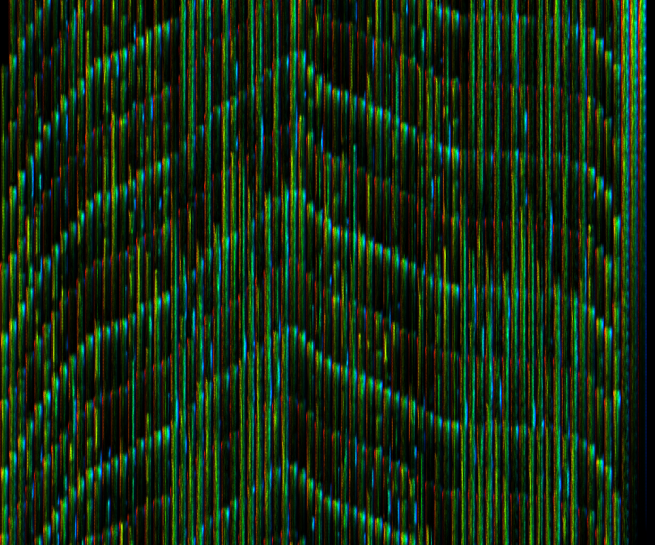
Once the tempo of music is known [1, 2], it becomes fairly simply to extract rhythmical information. This is done by summing together all consecutive measures from the song. This leads to a cyclic pattern that contains the average content of a sample.
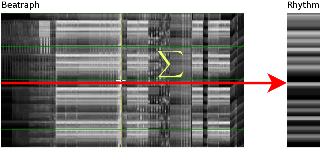 How the energy content of the song,
visualized as beatgraph can lead to a rhythmical pattern
How the energy content of the song,
visualized as beatgraph can lead to a rhythmical pattern
|
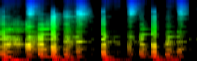
The result of such superposition of all measures can be heard below. In this case the patterns for the songs 'It Began in Africa (Chemical Brothers)', 'What are you waiting for (Gwen Steffani)' and 'All that she wants (Ace of Bass, Banghra remix)' are presented.
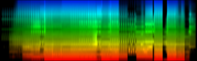
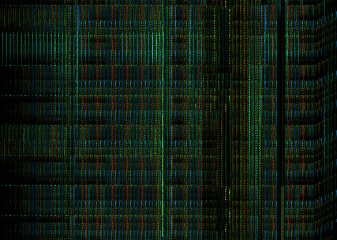
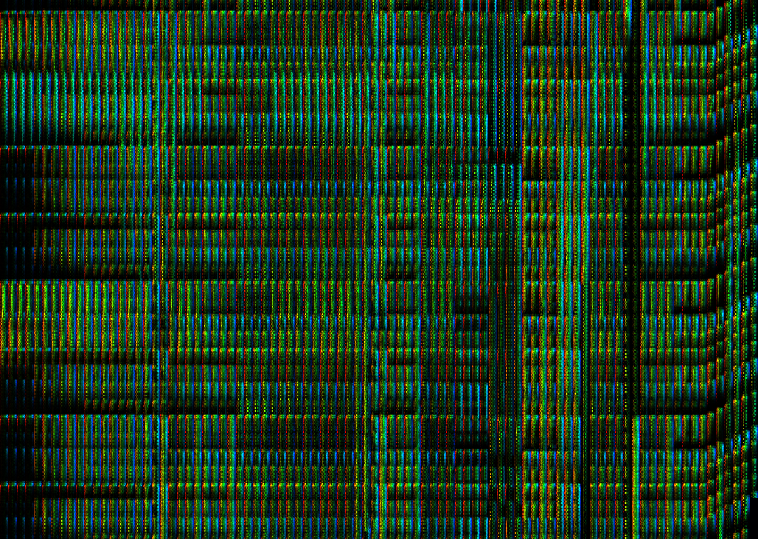
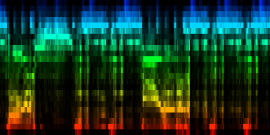
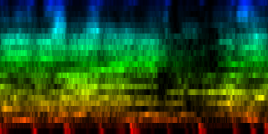
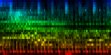
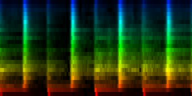
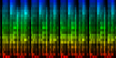
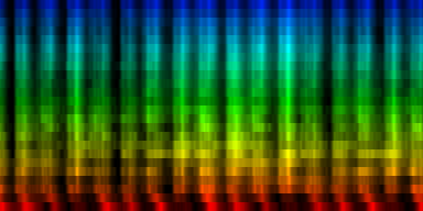
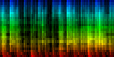
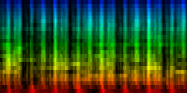
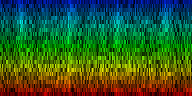
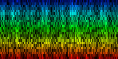
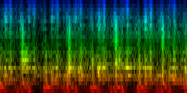
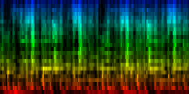
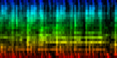
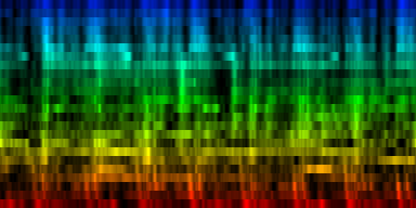
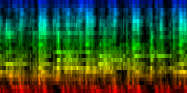
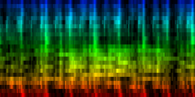
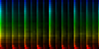
What is directly apparent is that we obtain a disproportionate amount of bass in many songs, while the melodic lines and hi-hats are lost. It is in other words, insufficient to just sum together all energy because a hi-hat often appears at different places (between bass-drums) and because jitter between different locations will favor one frequency over another. To account for this effect the use of a bark psychoacoustic scale [3, 4] is a valuable technique. Before summing together the various measures, the frequency content should be obtained. This no longer leads to samples that we can readily understand, but it will be able to separate hi-hats from basses and so forth. This is visualized below.
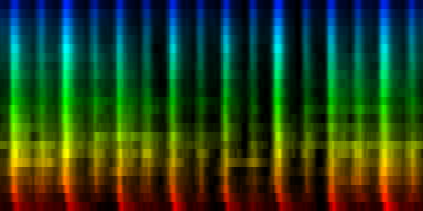
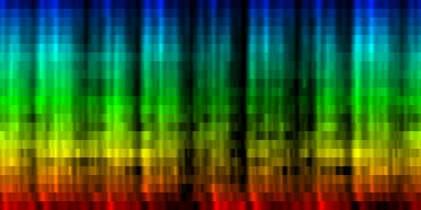
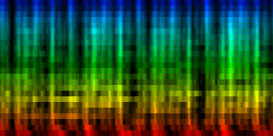
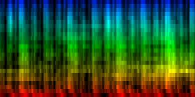
| ||||
| To extract the rhythm pattern of a song, we first convert the song into its 24 psychoacoustic bark-bands, after which we sum together all individual measures and obtain the 'average' measure. The red color are low notes, the blue color are hi notes. |
The second improvement on pattern extraction lies in the realization that each extracted pattern -if done naively- results in patterns of different size. E.g: one measure at 120BPM is around 2 seconds music, or 88200 samples, while a pattern of a 160 BPM song will only be 1.5 second or 66150 samples. To make it possible to compare patterns we must also fit them all to the same size. E.g: scale each pattern down to 256 samples per measure. (which offers a resolution of 1/64 note)
The general layout of a pattern extractor is thus a) to extract for each 1/64th note from each measure the frequency content, b) rebin the spectrum into 24 bands and c) sum together all these bands across all measures.
Triplets
Because we extract measures of which we don't know what time signature we talk about, it is necessary to be able to capture the finer points of for instance 3/4 measures; in this case each measure will only have 3 bass-drums, and the resolution we choose should allow the accurate placement of each of these beats. In a pattern containing 64 ticks, it is impossible to place those beats properly since we would need to place them at positions 0, 21.3... and 42.6...
A second consideration with respect to to the pattern resolution is that each extracted measure should be able to detect differences between 1/32 notes, meaning that we would like a resolution that can also capture 1/64 notes
A similar problem exists for the representation of triplets. (A 1/8 triplet are three notes played in a timespan of 2/8 notes). Because we want to represent 1/16th triplets and also changes from one triplet to another we might need to be able to store 1/32th triplets correctly. The necessary resolution for 1/16th triplet is the time necessary for 2/16the triplet divided by three, which gives 0.04166.... note, or when talking about 1/32th triplets 0.0208333... note. To bring this in a sensible range, we will need a resolution of 1/48 note
To combining these various resolutions, we need to find the smallest period that can represent each resolution (1/64note and 1/48 note). This is 1/192th note. 1/64=3/192 and 1/48=4/192.
Now, the difficulties arise of course if a measure only has 3 beats per measure, meaning that the 1/4th notes and 1/8th notes will also have different lengths. This is demonstrated in the following figure where we assume a certain number of ticks per measure and check whether we can represent each of the wanted notes.
| ||||||||
| Various resolutions per rhtythmical pattern and their capability to capture various notelengths and their triplets if a pattern contains 3 or 4 beats per measure. |
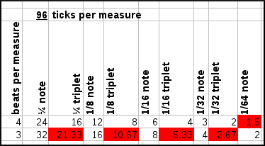
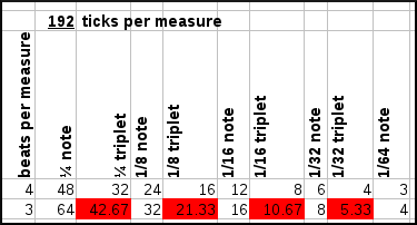
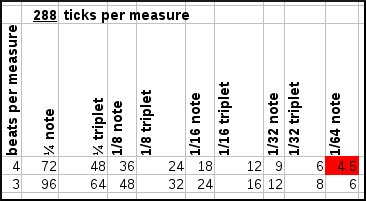
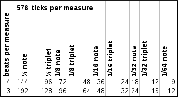
As can be seen from the above graph, the use of 96 ticks per measure leads to substantial difficulties encoding triplets in a 3/4 time signature, but has no problems encoding anything up to 1/32th triplet in a 4/4 time signature. At 192 ticks per measure, we solve the latter problem but still cannot encode triplets in 3 beats/measure time signatures. At 288 ticks per measure we can represent everything, except for 1/64th notes in a 4/4 time signature. To solve that we need to up the resolution to 576 ticks per pattern.
Because the need to encode 1/64th notes is maybe not required since we will be able to detect changes in 1/32th notes through the 1/32th triplets, it seems sufficient to use 288 ticks per measure.
[On a side note, while investigating the use of 1/64th notes I stumbled across a blog entry, titled 'Hats off gentleman' [5], which delves into a composition that requires tuba players and tenors to play/sing 1/64th notes :-)]
Although it is already clear that the frequency of each tick and measure should be extracted. That is, we need to divide each measure in 576 ticks and calculate the energy content of each of the 24 bark frequency bands, it is maybe useful to shed some light on this through a small calculation
If the tempo of a song is 60 BPM, then the length of 1 beat is 1 second, and the length of 1 measure will thus be 4 seconds, or 176400 samples. Each tick will consequently be 176400/576=306.25 samples, which means that, if we were only to take those 306.25 samples, we would have a frequency resolution of 144Hz. If the tempo was 90BPM, then each tick would only have around 200 samples left, which would lead to a accuracy of 216 Hz. That would merge the first few bark bands into one entry, which might be unwanted. Secondly, the extraction of the frequency content should use a Hanning window, so it makes sense to extend a Hanning window over each position we look for and double the windowsize. That would lead to windowsizes of 600 and 400 samples respectively; which is still quite low, but not underrepresented.
Given these bounds, it is further useful to ensure that we have a a power of two, since that tends to speed up calculations somewhat; leading to a windowsize of 512 bytes. A valid concern is now, whether the crude approach at lower frequencies does not lead to problems when mapping towards the psychoacoustic scale.
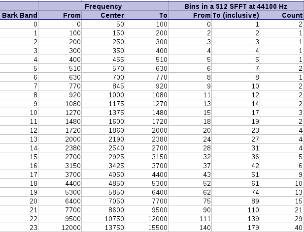 Mapping a 512 sample long SFFT at 44100 Hz towards the
frequency bands as deinfed by the bark psychoacoustic scale.
Mapping a 512 sample long SFFT at 44100 Hz towards the
frequency bands as deinfed by the bark psychoacoustic scale.
|
The requirements for a good extraction tool would be to be able to differentiate the appropriate accents and not trigger at random moments
Testing Windowsize versus Tickresolution
To test the above assumptions we set up a spectrum/tick based representation that would rely on 288 ticks per measure. The particular song we worked with was Horse Power (Chemical Brothers). We tested a variety of windowsizes from 512 to 8192.
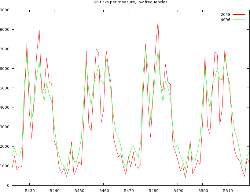
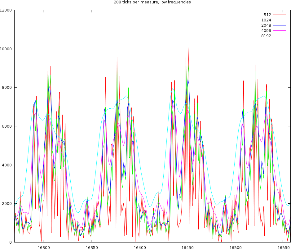 The channel content of 4 beats for low frequencies. We used windowsizes of length 512, 1024, 2048 and 4096 samples
|
The above figure shows 4 beats. At the lo channel with would expect each beat to be a nice Gaussian bump. That is however not what we observe. Only the windowsize of 8192 satisfies this vague requirement. All other window sizes oscillate within a beat. The worst of them are windowsizes of 512 and 1024 and 2048 samples.
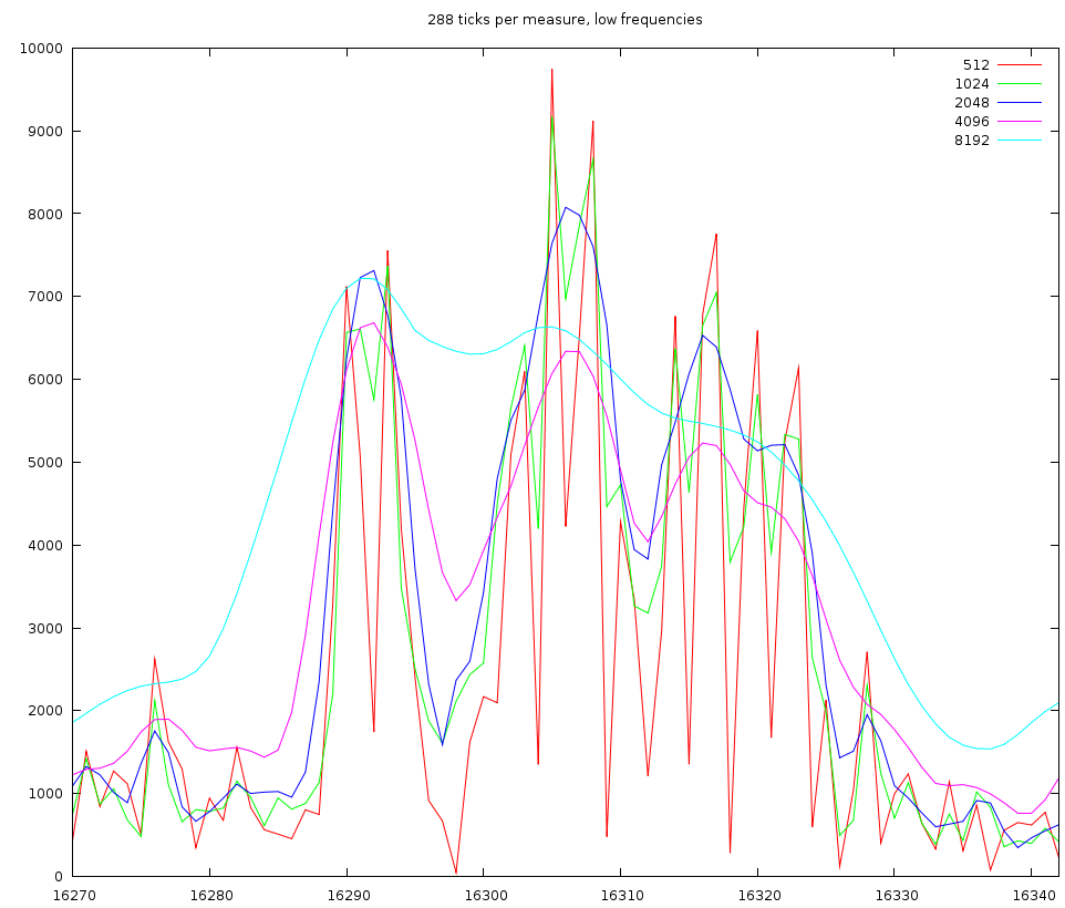 The channel content of 1 beat for low frequencies. We used windowsizes of length 512, 1024, 2048 and 4096 samples
|
If we look into one beat, then we find that these oscillations are at 1/96th notes. This is very unlikely and given that the oscillation is present throughout the signal, regardless of the presence of a beat or not, we must conclude that this is mainly an artifact of the samples used in this song; which leads to an important point: if we sample the energy content too detailed we will start finding events and notes back that belong to the content of other events. This is unwanted.
| ||||
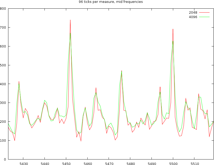
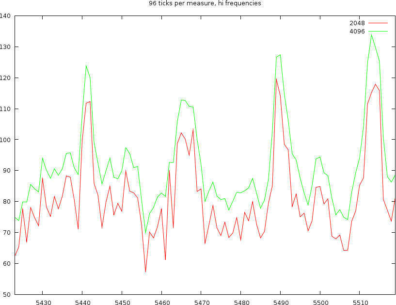
| Middle and hi frequencies using windowsizes of length 512, 1024, 2048 and 4096 samples |
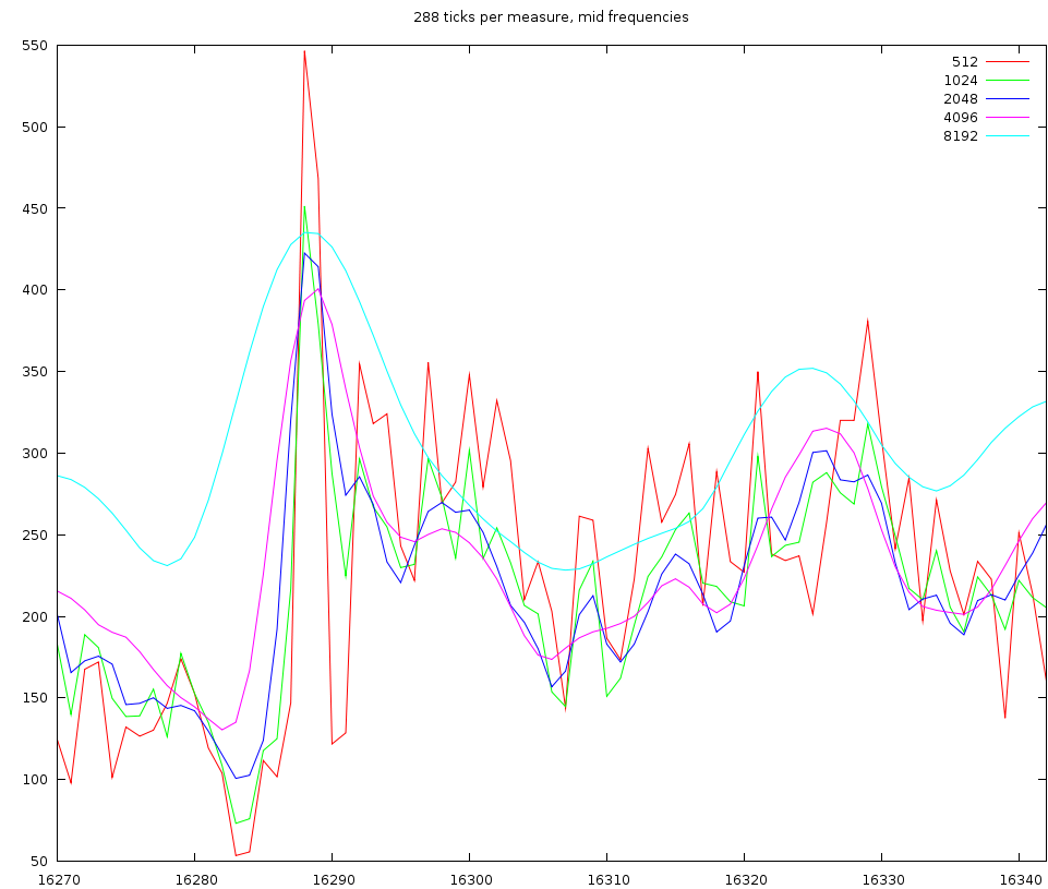
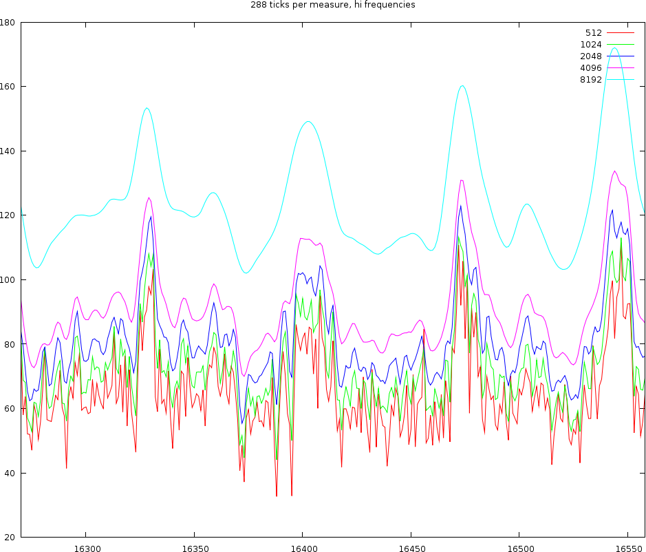
If we now look at a middle and a hi channel we find the same oscillations back. So it is clear that we cannot use windowsizes of 512 or 1024 samples. That leaves windowsizes off 2048, 4096 and 8192 samples.
Looking at a windowsize of 8192 samples we find that the two bumps are spread 1/8th note. Anything in between seem to have been lost. The very smooth nature of this windowsize is also apparent in the high channel, where it can barely capture the various oscillations. So this windowsize, regardless of the amount of ticks we use, is too wide to be useful. This leaves 2048 and 4096 samples.
In the plot left we also see that while the 8192, 4986 and 2048 lines are aligned at the first beat. 1/8th note further (right of the graph) we find that depending on the windowsize a certain positional bias comes into play. The 8192 windowsize has a distance of 1/8th note. The 4096 windowsize has a distance of 1/7.7 note. The windowsize 2048 has a distance that cannot be determined since we do not know what target point to choose.
In the same plot the oscillation of the blue line (2048 samples) has certain positions that are played at 1/48th note, which are 1/32th triplets.
We also find that an event in one channel will tend to affect other channels as well. This is especially true for bassdrums. They are not only low frequency events, they almost always contain all other frequencies as well.
So from all these considerations we find that it is useless to have a very high tick resolution. That resolution was necessary to be able to capture triplets in 3/4 and 4/4 time signatures, but now we find that songs might not be that simple to analyze. The best option at the moment is a) first to reduce the tick resolution to something like 96 ticks. This will at least be able to capture 3/4 time signatures and 4/4 time signatures but will not be able to encode every note we might wish (e.:g 1/64th notes, or certain triplets). See the above table.
We considered the possibility to generate two output maps. One with 64 ticks per measure (when the time-signature is 4/4) and one with 48 ticks, (for situations where the time signature would be 3/4. We did continue along this potential avenue.
Working with 96 ticks per measure
The first problem is still whether we choose 2048 or 4096 windowsizes. At 45 BPM, one measure is 5.3 seconds, or 235200 samples. Dividing by 96 gives 2450 samples. So, we could expect that the 2048 wide window will loose some information (sometimes), but this might lead to a better accuracy and no crosstalk between consecutive ticks.
| ||||||
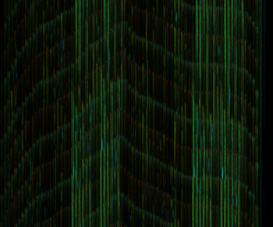
| The same song as shown in previous graphs but with a tick resolution of 96 ticks/measure. The same 4 beats are shown at windowsizes of 2048 and 4096 samples |
If we look into the time covered by a windowsize of 4096 bytes then we find that it covers about 96milliseconds; which means that at high tempos this will already cover half a beat ! We certainly don't want to have that, so we will be using a windowsize of 2048 bytes.
Stride
Given that we could position a tick always 'around' a certain position, it was not entirely clear how to deal with this problem. If we would always rigidly place it at the expected position, small tempo drifts might lower the frequencies and slowly move all information from one tick into the next. During this process the average tick content would be lower since the energy would be spread out over two ticks. That might potentially distort the outcome.
A first approach we used to solve this is to test multiple shifts and select the results that provide for the greatest differential in the data.
A second approach we used is to calculate the content of each channel multiple times by adding a random jitter to each expected position. That didn't really improve the results.
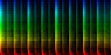
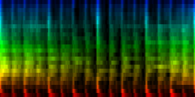
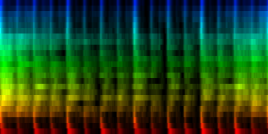
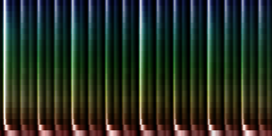
Appearence of a spectral beatgraph
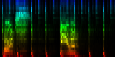
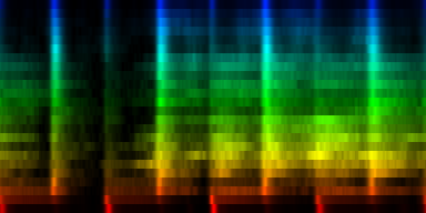
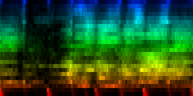
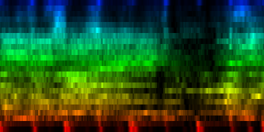
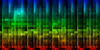
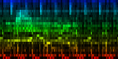
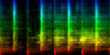
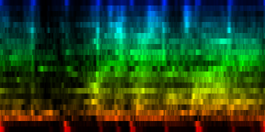
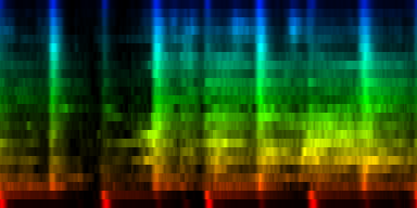
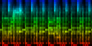
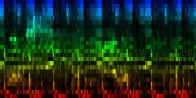
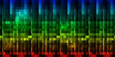
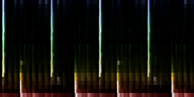
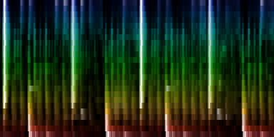
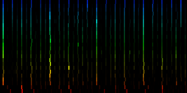
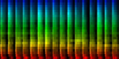
At this point we have enough data to present some results, relying on 384 ticks per pattern and a windowsize of 2048. In the images the measures are stacked next to each other, while the content of a measure is shown from top to bottom. Two normalization schemes have been used. The first normalizes each band across the entire song. The second image, normalizes each band for each individual measure. The colors are still the same as the above rhythm extractors: red is the lowest bark band. Blue is the highest bark band.
| ||||||||
| spectral beatgraphs of the song Griechischer Weinn - Udo Jurgens (top-row) and Horse power - Chemical Brothers (bottom row) |
Although in these picture we can clearly see when the guy starts singing, it is not yet clear whether preserving this information is sufficiently accentuated to allow a neural network to decide in favor of the lower tempo. A second observation regarding the griechischer Weinn ist dass the bassdrums and the bass can now be separated properly. This might, form a basis for a proper classification later on.
Tempo changes
Most humanly played songs drift around their average tempo. This 'jitter' or 'drift' is both a problem and not a problem. As already explained in [2], such jitter does not sufficiently affect the tempo measurement algorithms to be of concern. However, if we want to extract the rhythmical information and later on put such rhythmical patterns into a neural network, then this jitter must be removed (even if it only affects 5% of the songs, these 5% are sufficiently worthwhile to try to reclaim).
Strategy 1: Align towards the previous measure
The first algorithm we tested to deal with this problem is a form of cumulative superposition. We would take the first measure and store it into the pattern. Then we would take the next measure and align it towards the previous measure, and then sore it into the pattern. After that we would shift to the next measure and with each step we would always align towards the last seen measure, while at the same time building up the pattern
This strategy doesn't work too well because and alignment to the previous buffer might throw off the measure-offset in empty spaces and then, when the new measures are picked up again, would interleave two different measures through each other. Instead of 4 beats, we would count 4 beats (from the first half of the song) and interleaved between them, possible 4 other beasts (coming from the second part of the song).
Strategy 2: Straighten out the song first
We did create an algorithm to straighten out a song, so that it will follow the appropriate tempo. This was recursively done by taking the entire song and calculating a point in the middle of the beatgraph that will slant all measures up/down as to obtain the biggest overlap. This process is recursively repeated until we have no measures to shift anymore.
| ||||||
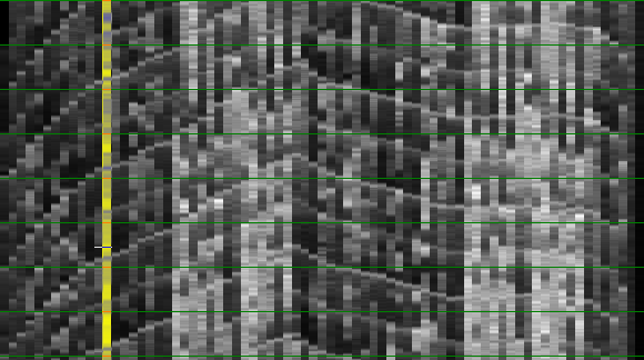
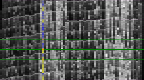
We currently use linear interpolation. With the restriction that the slant of a line cannot exceed 10% we still have a potential for relative strong pitch changes. Especially at each node where we change the slant. Below is a sample of a normal song and the flattened version. The result of this flattening is an output that brought all measures in sync, without preserving accurate pitch. Consequently we will only be able to use this output to recognize time signatures and rhythmical information.
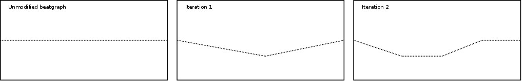 Straightening out a song is
done by finding the required repositiongin of the middle point
as to obtain the lowest autodifference. This process is then
repeated for each of the resulting segments until we cannot
calculate the autodiffrerence anymore
Straightening out a song is
done by finding the required repositiongin of the middle point
as to obtain the lowest autodifference. This process is then
repeated for each of the resulting segments until we cannot
calculate the autodiffrerence anymore
|
Strategy 3: Align towards the acummulated pattern
Another strategy was to build up the pattern as we look into each new measure, but instead of aligning each measure towards the last seen measure, we align it towards the pattern-so-far. This approach was quite appropriate and between 2006 and 2010 was in use in BpmDj [6, 7]. The code for such a rhythm pattern extractor is given below
for(int measure = 0 ; measure < measures ; measure++)
  {
    // read data
    long int pos = measure * measure_samples;
    fseek(raw,pos*sizeof(stereo_sample2),SEEK_SET);
    int read = readsamples(measure_audio,measure_samples,raw);

    for(int a = 0 ; a < 8 ; a ++)
      {
	// take the appropriate data
	int s = a * ( measure_samples - 8 )/ 8;
	assert(s + 8 < measure_samples);
	for(int i = 0 ; i < 8 ; i++)
	  buffer_fft[i]=measure_audio[i+s].left+measure_audio[i+s].right;
	// convert to spectrum and normalize
	bark_fft2(8,measure_freq[a]);
	for(int i = 0 ; i < 4 ; i ++)
	  {
	    float8 v;
	    v = measure_prot[a].bark[i];
	    assert(!isinf(v));
	    v = tovol(measure_freq[a].bark[i]);
	    assert(!isinf(v));
	    measure_freq[a].bark[i]=v;
	  }
      }

    // find best rotational fit towards prototype
    float8 m = HUGE;
    int a = 0;
    for(int p = 0 ; p < 8 ; p++)
      {
	float8 d = 0;
	for(int y = 0 ; y < 8 ; y++)
	  {
	    int z = (y + p)%8;
	    for(int b = 0 ; b < 4 && d < m; b ++)
	      {
		float8 v = measure_prot[y].bark[b] / measure;
		float8 w = measure_freq[z].bark[b];
		d += (v-w) * (v-w);
	      }
	  }
	if (d<m)
	  {
	    m = d;
	    a = p;
	  }
      }
    phases[measure]=a * ( measure_samples - 8 )/ 8;
    // add the rotation to the prototype
    for(int y = 0 ; y < 8; y++)
      {
	int z = (y + a)%8;
	for(int b = 0 ; b < 4 ; b++)
	  measure_prot[y].bark[b]=measure_prot[y].bark[b]+measure_freq[z].bark[b];
      }
  }
Although this strategy works like a charm, there is a potential error due to the fact that all measures coming after the currently build-up pattern will try to create the same pattern all over. Thereby the algorithm might become biased towards the first measures in the song.
To compare measures we tried both the L2 and |abs| norm. Both resulted in surprisingly similar results.
Dealing with Tempo changes
Most songs drift because the artist in question didn't follow a strict metronome. This means that -as already explained- we will have measures that shift up and down in the beatgraph. There is however a second aspect which is that certain measures might be slightly shorter/longer than other measures (otherwise, one would not notice this drift).
To deal with shorter and longer measures, it is quite useful to attempt to modify the measure under consideration slightly, with for instance a potential shortening or lengthening of 10% and then perform the alignment towards the pattern buffer. This will thus lead to a search algorithm that attempts to match the tempo and the offset of each measure towards the average expectation
An experimental algorithm that used this offset first, scale then, and offset again showed us that an allowed 10% drift is quite a stretch. In general at most 1/32 measure difference is noticeable between measures (which is a 3.125% speedup/speed down already). Once we reduce the allowed tempo change to 1/32 note, the algorithm also performs much faster than when using the 10% allowed tempo drift.
Normalizing Rhythmical Patterns
In this section we investigate the following problems that might affect the calculated distances between various measures.
- Sound color The various frequency bands have different energy levels. As a rule, low frequencies have a higher energy than high frequencies. The mean energy per frequency band is dependent on the sound color of the song.
- Cross talk The Fourier analysis is subject to a certain crosstalk between channels. When a sharp event triggers then all frequency bands are affected. We might want to find a solution to this problem as to improve the specificity of each tick/frequency data point.
- Accents The event strength distribution is 'accented', with that we mean that it has a musical meaning that something is played at 75% of its maximum amplitude or not.
- Noise affects metric The presence of noise increases the variance (width) of the event strength distribution. That will lead to larger distances than necessary, when comparing two measures.
- A song is a composition Most songs are compositions, which means that not always the same rhythm is present. Empty spaces (devoid of any rhythm), and places where the lead guitarist/singer is going off the rails might affect the retrieved rhythm pattern.
- Echoes echo effects will spread out a single event over multiple ticks. This affects again the energy distribution.
Normalizing Sound Color
The average spectrum (the sound color as it is commonly called) affects the presence of each of the frequencies, which in turn, since we add all the frequencies together, will affect the full rhythm pattern. The result is that if we were to compare multiple measures we would mainly be measuring the difference between the sound color of the songs involved.
- min-max normalization We can normalize each band so that its maximum energy would be placed at 1 and its minimal energy at 0. The advantage of this method is that it is simple and fast. The drawback of course is that it would sometimes lead to a strong amplification of noise in bands that had almost no energy. That was however remedied by not calculating the frequency band up to 22050 Hz and skipping that last one. However, a second drawback was that such normalization would still not normalize the sound color.
- min-mean-max normalization mapping the maximum energy of a frequency band to 1, then mapping the mean to 0; and then mapping the minimum to -1.
- mean-max normalization Normalize the average band-spectrum to 0 through subtraction of the mean, and then normalize the maximum energy to 1. That would offer two pieces of information at the same time and has been successfully used in BpmDj. [6, 7]. I'm not a fan of this method since it throws away potentially valuable information).
- ratio-mean and log-ratio-mean normalization We can normalize the content of each band with respect to the measured average spectrum. Thus, divide the frequency content of each tick by the average frequency energy. In this case we can attain unlimited large values, if the mean is sufficiently close to 0. This would imply that we might need a logarithmic interpretation of this division. It would however solve the sound color problem.
- perfect spectrum normalization We could try to normalize towards the 'perfect spectrum', [8], but in that case we would merely affect the weighing.
- rank the energy The reasoning behind this approach was that the distribution of the energy landscape is dependent on the sound color, however, the echo characteristics will lead to different energy histograms. To normalize these the only sensible approach seems to be the use of a ranking process on each band.
- log normalization a technique that everybody probably will think about is the conversion of the energy to their perceived volume through an energy->dB conversion.
Normalizing Crosstalk
When a bass-drum hits, not only the lower frequencies are affected, but also all higher frequencies. This single event will thus lead to matches or mismatches at multiple locations. Therefore we considered the possibility to bring this single event back to its most prominent frequency.
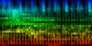
tick-min-max normalization A simple method here is to also normalize each channel individually. This would of course directly affect the mean energy of certain frequency bands, so we might need to repeat the frequency normalization then again. After a number of such horizontal (across ticks) and vertical (across frequencies) normalizations, we would obtain a rhythm pattern. Below is the output of our favorite Horse Power song again, once with and once without vertical normalization
| ||||
| Vertical normalisation (that is normalization oif the frequency content within each individual tick) versus non vertical normalized patterns |
In this little experiment we directly see that this type of normalization is problematic because a) when a bassdrum hits, it will affect all frequencies, but when we then normalize it to a range of 0:1, we loose all energy present in that beat. Vice versa we find that b) places that have no energy whatsoever will suddenly appear as beats since all the emptiness will get amplified to 0:1 as well.
In conclusion, vertical normalization is unwanted and will very likely not produce anything of value since we loose all energy accents
A Crude Measureument of a Pattern C.I
In most song, aside from the repetitive rhythmical pattern there are also passages that might or might not be present, or rhythmical effects that contain noise, and of which the energy of the event is not always the same. Such variances will lead to a less strong presence of these events.
To study this we calculated aside from the standard pattern, also the deviation of the song towards the pattern (variance), the skew and kurtosis factors.
| ||||||||
| The various distribution properties of the energy associated with each event. (Gw) |
| ||||||||
| The various distribution properties of the energy associated with each event. (Hp) |
As can be seen, the target pattern contains quite some information and also the variance provides useful information. The two other properties are of much less useful nature. As illustration we create a number of graphs that would use the average and absolute value to set lower and upper bounds on what we could be expecting. Which of these two (minimum versus maximum expectation) are useful is unclear at the moment.
| ||||||||
| Our Gw song, the average pattern, the abs deviation of that pattern and the upper and lower bounds of the expected rhythm, pattern |
| ||||||||
| Our Hp song, the average pattern, the abs deviation of that pattern and the upper and lower bounds of the expected rhythm, pattern |
Selecting good measures
The song composition might also affect the distribution of the event strength. For instance a singing guy present from first to last measure (or in case of ego tripping guitarist: a lead guitar), and then somewhere in between we have a few measures of rhythm. In such cases, the rhythm pattern will be drowning in other noise.
A solution might be to actively select only the patterns that are sufficiently close to the pattern buffer itself. By doing so, we will automatically ditch empty parts of the song.
| ||||
| Our Hp Song. The difference between selecting close measures and realignment and not. |
| ||||
| Our Gw Song. The difference between selecting close measures and realignment and not. |
Accent Distribution
The normalization procedure as explained up to now (min-max or min-mean-max) might not be sufficient to normalize between songs. The problem arises from the presence of echoes. Such type of effects tend to spread out the energy and thus lead to different energy distributions in a song. Therefore it is necessary to understand the energy strength distribution (Which we will call the 'Accent Distribution') per channel so that we may find a better normalization method as to enable the correct comparison across different songs. Ideally, we would like to bring the standard energy distribution per pattern in line with a required energy distribution.
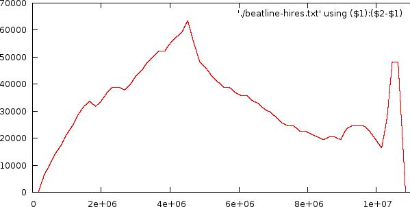
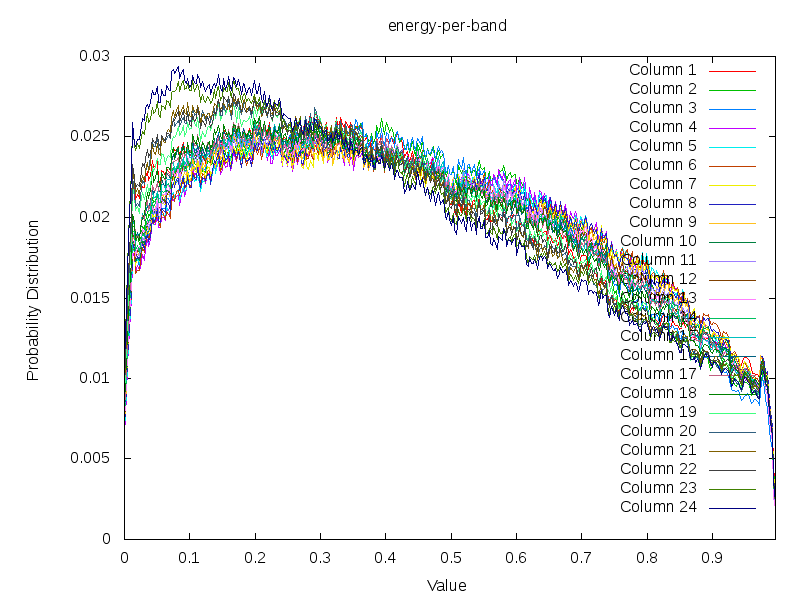
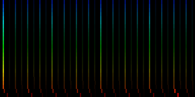
 Taking the energy content of 430 song, whereby each band has been minmax normalized,
shows the following log normal distribution
Taking the energy content of 430 song, whereby each band has been minmax normalized,
shows the following log normal distribution
|
What is interesting in the above plot is that most of the signal of a song is close to 0. This means that the events that interests us are hidden away in the right tail. Aside from this, we also see the typical pattern of a log normal distribution. The low energy channels also have a bit of accenting going on. Slightly higher channels seem to behave slightly more as a Gaussian than a lognormal distribution. In general the tendency is somewhere between a log-normal and a log distribution.
Log normalisations
One might assume now that 'log normalizing' these values by might make psychoacoustic sense. At least the belief is often that taking the log of an energy results in a measure that reflects how we perceive changes in sound strength. (E.g: a doubling of volume is a 3 dB increase, or 6, depending on what scale is used). Sadly enough, the author of this paper is a strong anti-log fan. I don't like to use them because they make no sense. I do understand them though, the only problem is that I often have problems normalizing energy spectra to a 'perceived volume' using a log-scale (which is what is typically done when converting to dB). My problem comes from the fact that it is impossible to convert low and 0 energies to a measure that reflects what we here (- infinity ???). So, that doesn't ring quite correct to me. One could consider the use of a log towards the mean energy of the band. That might make some sense, but in general is difficult to work with due to arbitrary cut-offs.
Secondly, the value are often already lognormal
distributions. Taking a second log will not 'normalize' them at
all. Instead, one should consider 'exponenting' them.
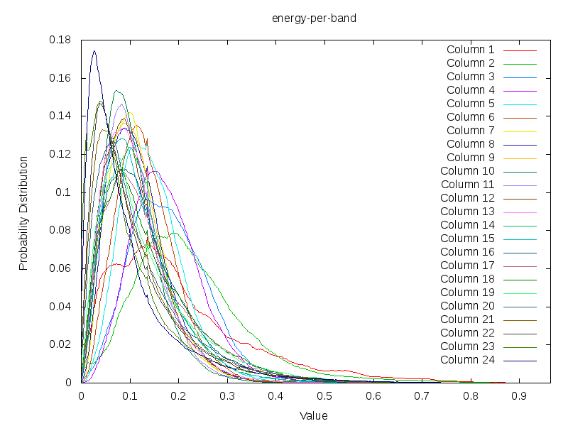
The effect of min-mean-max on the Accent Distribution
 The effect of min-mean-max normalization on the accent distribution. Taking the energy content of 430 song, whereby each band has been subject to the min-mean-max normalization.
|
In the above plot we've plotted the energy strength distribution if we use a min-mean-max normalization. The strong cutoff at 0.5 is because the mean is for each pattern translated to this position. So we find that we have a relative large amount of information present above the mean (not unexpected given the previous graph that contained a lognormal distribution, with more weight on the right side). A second observation is that the slant of each frequency band is quite similar. This in contrast to the previous graph. So there is something to say about bringing the mean to the same position for all songs. However, it still does not make it possible to bring the data at the appropriate band. To do so, we will for each side again bring the mean to a fixed value and normalize according to such a pattern
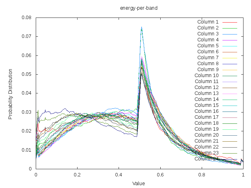
Ranking Accents to generate a Uniform Accent Distribution
 Taking the energy content of 430 song, whereby each band has been redistributed to follow (more or less) a uniform distribution. The non-uniform appearance of this plot is due to the fact that each pattern (each of the 430) was individually normalized before adding them all together. The resulting curve is a result of the law of great numbers, however in this case, the unnatural (unnormal) distribution of beats and empty spaces lead to a slightly less normal normal distribution.
|
Quantile Normalization
Because the ranking approach would weigh low accents more heavily that strong accents (which is wrong if we compare two patterns using || or L2), we preferred to stay close to the actual distribution using in music. This could be solved by quantile normalizing the different energy bands. By using the probability distribution across all songs as target distribution we were able to 'clean up' various songs with highly unbalanced distributions.
| ||||
| A song (Mind Rewind - Plastikman) that had a highly unbalanced accent distribution before and after quantile normalization. |
Some notes on the technical aspect of quantile normalization: a) the target distribution must be calculated such that no single song has an overly strong weight in the result; which means that the integral of the value (not the probabilities) must be 1 as well. b) to create a smooth target distribution it is necessary to smooth out the cumulative distributions of each individual songs before adding them.
Echoes
Echoes lead to a blurring of events. This is good because a distance metric between measures can be off by a tick or two. It is bad however, since the width of the blurring also affects the distance. Ideally, we would like to have each event have the same width. That means that we will need to convert a rhythm pattern to a collection of single spaced events joined with an impulse response that will convert that frequency band back to its original.
Requirements on the impulse-response
To understand how we can solve this it is necessary to explain some of the detail of convolution: by taking the spectrum of a signal (forward Fourier transform) and then multiplying it with the conjugate spectrum of another signal, we create the spectrum of the convolved signal. If we then perform an inverse Fourier transform, we will find the convolved signal. As an equation: F_inv(F(A).F(B)*) = A x B.
In the above, A is known (it is our energy representation of a specific bark band). B is not known. We do however know that it should behave somewhat as an exponential decaying process. An attempt to use this type of deconvolution based on lognormal distributions did not succeed. In practice we found that the energy decay is dependent on the frequency band we are investigating; and that it is not a lognormal process at all. Very often we found tailing frequencies that could not be accounted for using a lognormal distribution.
The last solution we came up with, was to find peaks in the convoluted signal and then assume that the 'impulse response' around this particular element is a strict decreasing function (to the right and left) and model that particular peak as such. Repeating this process sufficiently leads automatically to a nice collection of event entries and solves the problem of echoes and standard frequency distributions quite well. c) if we perform this step, it is necessary that the means and variances of the target distributions across frequency bands is aligned, then we don't need to 'fix sound' color issues later on anymore'.
| ||||
| Happy pills (Younger Brother) with and without event extraction. |

Results
| Technique | Sound color | Cross talk | Accents | Noise | Echoes |
| min-max | affects metric | still present | preserved | increases distance | affect metric |
| min-mean-max | does not affect metric | still present | more weight is given to low energies | increases distance substantially (given that low energies tend to be amplified) | still present |
| mean-max | does not affect metric | still present | preserved only if larger > mean, which is to be expected | increases distance somewhat, but since anything below the mean has been cut away, the effect of noise is less apparent. | still present, but slightly cut in number of ticks due to the cutoff |
| ratio-mean | does not affect metric | still present | preserved, but might lead to arbitrarily large energies | might be amplified (above the mean), or reduced (below the mean) | affected arbitrarily |
| log-ratio-mean | does not affect metric | still present | probably preserved in a sensible manner. However, the presence of 0 might lead to -inf 'volumes'. | given the nonlinear redistribution, then noise will be amplified and lead to larger distances. | affected arbitrarily |
| log-energy | affects metric | still present | The presence of 0 might lead to -inf 'volumes'. Otherwise accents are readily comparable based on their psychoacoustic appearance | Noise will be amplified and lead to larger distances. | Arbitrarily affected |
| tick-min-max | does not affect metric | removed | brought completely out of balance. Empty areas will become large volumes and high energy beats will become low volumes. | Substantial amplification of noise, leads to larger distances. | Arbitrarily affected |
| ranking energies | average frequency energy will fall in middle ranks | dependent on the interaction between multiple ticks. Will be affected nonetheless. | nicely reduced to rank numbers. However, the rank distance does not reflect our sense of volume change | amplified, due to the many 'near 0' in most frequency bands. A uniform distribution will bring most of these zeros to larger numerical values. | will widen the events, but the echo strength will be ranked as well |
| quantile normalization energies | average frequency falls at the same position | still be present. | accents are comparable now. On average, the hold their own position and no single accent strength is favored over others (as compared to ranking) | will not be amplified, unless there is much empty space in that particular frequency band. | will all be normalized to the same target distribution |
| absdev | depends on the main calculation | not removed | not directly modeled, but events can be better understood. | can be removed by choosing the lower bound of the C. | Will be slightly removed due to a lack of certainty in echo-areas |
| Peak finding | Removed | Stays | Stay | Removed | Removed |
Normalizing Rotation Offsets
An important aspect of Dj software and tempo categorization is the ability to compare measures between each other. This is sadly enough not such a straightforward problem because one must after defining a metric (L2 or || will do), also find a sensible alignment algorithm so that the measures can be compared element by element.
Measure Alignment
If one has two measures: A and B, then the distance between those two measures can be defined as follows
- Set bestmatch to infinity
- Set required_rotation to -1
- Calculate for each possibility position i in the rhythm pattern A[i]-B[i]
- Sum all these values together
- If the summed value is smaller than the best match, then set the best match to this value and set required_rotation to the current rotation
- Rotate B one tick and increase the current_rotation with one
- Repeat this process until all possible rotations have been tried.
In code, the algorithm is probably more transparent:
float distance(float* A, float* B, int rot)
{
  float d=0;
  for(int i = 0 ; i < floats_per_pattern; i++)
    {
      float a=A[i];
      float b=B[(i+rot)%floats_per_pattern];
      d+=fabs(b-a);
    }
  return d;
}

int bestfit(float*A, float*B)
{
  float error=HUGE;
  int answer;
  for(int rot=0;rot<ticks_per_pattern;rot++)
    {
      float d=distance(A,B,rot);
      if (d<error)
	{
	  error=d;
	  answer=rot;
	}
    }
  return answer;
}
Although the above metric works quite well, it is a time consuming process and will only works between two rhythm patterns. This is bad since the training of a neural network or any classification process will expect some form of aligned data to be present. If the data can just be repositioned from one place to another, then we cannot expect solid results from future classification processes. Therefore, we set out to pre-align the measures towards a specific standard. The problem is of course the design of such a standard
A good alignment standard should
be able to report an offset for each specific rhythm it is presented withAll Known Rhythms against Noise
The first standard we came up with, was to take all known patterns and align them towards a noise rhythm pattern (devoid of any sensible meaning of rhythm). Once all alignments have been done, we would add them together into one new standard.
The idea behind this was that the final standard would be something towards which we could align any unknown measure. For instance, if we would have measure A, we could align A towards this standard S. If we would have another rhythm B, we could also align this towards this standard S. Afterward, the alignment of A towards S and the alignment of B towards S should be related somehow
| ||||||||||||||||
| A number of 'standards' generated by akligning all known information towards a noise rhythm pattern |
Weighted according to problematic twins
It turned out that the creation of a pattern as described above could produce a number of random standards, which was already a hint that the process didn't work fully. Mainly, because depending on the dataset used to train the standard, we would find a certain type of song to be ,ore present. Assume for instance that we have 99 4/4 rhythms and 1 3/4th rhythm. Simply summing together all known rhythms will make it impossible for the 3/4th rhythm to have any impact on th final standard. This will consequently lead to misalignments, for this particular type of rhythm (or that is what we could expect)
To continue working this out we needed to formalize what we were looking for. We wanted to bring similar measures to the same position. How could we formalize that ?
If we bring similar measure to the same position then this is with the aim that direct comparison between those two prealigned measures would be similar to a comparison that includes its own alignment. That is to say: if we have two pattens: A and B and a standard S. If we align A to S and B to S; Based on these two alignments it is possible to deduce an alignment between A and B. This deduced A to B alignment should be very closely related to the directly measured alignment between A to B.
Of course, the tricky thing is that merely obtaining the same offset is not sufficient. Actually the offset doesn't matter because certain patterns are self repetitive. We might as well have a similarly good alignment at other offset, not reported by the deduced alignment, but equally good. We are thus aiming to minimize the absdist(A,B_rotated_based_on_deduction) against the minimal distance we can achieve, given the best possible rotation between A and B. So, back to human terms: we are looking for a standard that will minimize for each potential pair of rhythms absdist(A,B_rotated_based_on_deduction)-absdist(A,B_optimal_rotation). Below the code is given for such a quality check of a standard
for(int test=0;test<tests;test++)
  {
    int a=random()%all.size();
    int b=random()%all.size();
    float* A=all[a];
    float* B=all[b];
    int A2S=bestfit(standard_now,A);
    int B2S=bestfit(standard_now,B);
    /* the outcome is checked by calculating the optimal alignment */
    float lowest_error;
    int B2A=bestfit(A,B,lowest_error);
    /* and what it is if aligned through the standard */
    int B2A_deduced=(B2S-A2S+ticks_per_pattern)%ticks_per_pattern;
    float actual_error=distance(A,B,B2A_deduced);
    avg_err+=(actual_error-lowest_error)/tests;
  }
To train such a standard, we started to sample from our pool of patterns and for each pair we reported the error that was introduced due to that combination. Both elements of that pair would then contribute their error as weight to the new standard. This process would be repeated and we hoped that this would eventually converge on something that was satisfactory.
| ||||||||||||||||
| The creation of a standard based on 'problematic pairs'. These are pairs that align between themseleves but cannot be resolved through the standard. |
The formal definition of the quality of our standard revealed that the process converged slowly and started to oscillate after a number of epochs. In general, the average error was around 57 pixels, with a maximum of around 790 pixels (the total number of mismatching pixels is 9216).
After 19 steps we started to observer that the standard started to aggregate much information at the same place, so we started to think along these lines to create a standard in a slightly different manner
Largest Energy Upfront
We implemented two variants of this algorithm. In the first, we find the tick that contains the largest energy spread over the 24 channels. In the second algorithm we gradually narrow down the bands we consider for maximum (this is in a real sense, a multi-rate maximum finder and refiner).
| ||||
| The average patterns generated from over 275 rhythms based on two different prealignment methods |
| ||||
| The average deviations generated from over 275 rhythms based on two different prealignment methods |
From the above results it is difficult to conclude whether the fuzzy or strict method is to be preferred. Looking at the strict average pattern, we find that of course we get all beats strictly spaced at 1/4 and 1/8 th notes. This is not unexpected. The question is how, will singing and other instruments be positioned.
The deviation plots show that the strict method provides for less uncertainty in the middle of the pattern, while the fuzzy method seems to place uncertainty evenly throughout the pattern. Which one of these is good is unclear. We could argue that such 'dead' areas in the pattern are useless later on, and if there is no variance and the rhythm is always the same: who would care ?
An argument against the use of the fuzzy method is that a low attack in certain rhythms might shift that rhythm half a measure, which might lead to the wrong conclusion during pattern analysis.
All in all it is unclear which of these two strategies is best. What is sure however, is that these two already form a good approach towards alignment standardization
How does such a pattern sounds like ?
To study the extracted rhythms we created a number of sound synthesized purely from the extracted pattern. The process relies on the perfect spectrum [8] to define the required energy per channel. Otherwise only noise is used to generate the sound fragments.
For each fragment we created sound fragments based on the perfect spectrum
- as the pattern was extracted
- after removing the background noise (mean subtraction and variance normalization)
- event extraction
| ||||
| Average pattern of 1078 songs. |
Conclusions
In this paper we discussed a large number of issues related to pattern extraction. We briefly list the useful conclusions we can draw.
- To represent a rhythmical pattern we need a resolution that can capture a wide ranges of notes (1/4th notes to 1/64th notes) as well as their triplets at a time signature of 3 or 4 beats per measure. This leads to a resolution of 576 ticks per measure. That is however insufficient for 7/8 and 5/8 rhythms. Our experience also shows that blurring of notes does not allow our algorithm to accurately extract notes at such high resolution.
- We tested the necessary windowsize to obtain sufficiently stable results. At 44100 Hz, a window size of 2048 sample is preferred, combined with a Hanning window. Oversampling certain positions by reducing the stride did not sufficiently affect the overall outcome to be of a concern.
- We introduced a beautiful new method of visualizing beatgraphs, called spectral beatgraphs.
- To extract the rhythmical pattern out of a song, one should use a pattern buffer that is filled incrementally with new measures taken from the song. Each measure is aligned towards the pattern buffer before it is added.
- This process can be improved by, after the first pattern has been generated, repeating it for only 50% of the closest measures. In this second phase, the patterns can also be stretched slightly. Our experience is that this stretching seldom occurs and that the main issue has been the offset between measures.
- The normalization of the energy content of each spectral band has been studied in great detail. The largest problem is initially the sound color. Second after that is the energy distribution due to echoes.
- mean subtraction and variance normalization removes the sound color aspect.
- So does the peak detection.
- To allow inter-pattern comparisons we need to rotate the individual patterns. Both L2 and || norm are sufficient.
- Pattern rotation is time consuming and can be avoided by prealigning them. Most useful is to place the highest energy first.
Currently it is still unclear whether
- Whether a fuzzy or exact 'largest-energy-first' alignment works best
- Whether the pattern without echoes is more useful than the pattern with echoes.
- Whether the absolute deviation adds any value at all to the extracted patterns.
Future Work
- An avenue of thought was the use of a ranking based event strength normalization before sending the data to the pattern buffer. Or even further: deconvolving the various frequency bands before sending it to the pattern buffer.
- Given the deconvolved signal and the normal signal, we can know calculate the impulse response necessary to bring the events back to the signal. This can be used as a further metric, or a better metric, in BpmDj.
- The generated average patterns do not take into account the 'uniqueness' of each individually added element. Which means that it will be biased towards the style of music that is most present in the data.
Bibliography
| 1. | BPM Measurement of Digital Audio by Means of Beat Graphs & Ray Shooting Werner Van Belle December 2000 http://werner.yellowcouch.org/Papers/bpm04/ |
| 2. | Biasremoval from BPM Counters and an argument for the use of Measures per Minute instead of Beats per Minute Van Belle Werner Signal Processing; YellowCouch; July 2010 http://werner.yellowcouch.org/Papers/bpm10/ |
| 3. | The Bark and ERB bilinear transforms Julius O. Smith, Jonathan S. Abel IEEE Transactions on Speech and Audio Processing, December 1999 https://ccrma.stanford.edu/~jos/bbt/ |
| 4. | Psychoacoustics, Facts & Models E. Zwicker, H. Fastl Springer Verlag, 2nd Edition, Berlin 1999 |
| 5. | Hats Off, Gentlemen http://www.fredosphere.com/2005/11/hats-off-gentlemen.html |
| 6. | DJ-ing under Linux with BpmDj Werner Van Belle Published by Linux+ Magazine, Nr 10/2006(25), October 2006 http://werner.yellowcouch.org/Papers/bpm06/ |
| 7. | BpmDj: Free DJ Tools for Linux Werner Van Belle 1999-2010 http://bpmdj.yellowcouch.org/ |
| 8. | Observations on spectrum and spectrum histograms in BpmDj Werner Van Belle September 2005 http://werner.yellowcouch.org/Papers/obsspect/index.html |
| http://werner.yellowcouch.org/ werner@yellowcouch.org |  |