| Home | Papers | Reports | Projects | Code Fragments | Dissertations | Presentations | Posters | Proposals | Lectures given | Course notes |
|
|
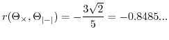
Correlation between the inproduct and the sum of absolute differences is -0.8485 for uniform sampled signals on [-1:1]Werner Van Belle1* - werner@yellowcouch.org, werner.van.belle@gmail.com Abstract : While investigating relations between various comparators and the inproduct we found that the inproduct correlates strongly towards the absolute difference when the domain from which the values are taken come from a uniform distribution on [-1:1]. This useful relation might help to speed up block comparison in content databases and can be used as a valuable tool to estimate the inproduct based on the absolute difference and vice versa
Keywords:
sum of absolute differences, sum of inproduct, landmark tracking, feature tracking |
1 Introduction
To compare two data-blocks (of size ![]() ), two easy implementable
techniques are widely used. The first is the summed inproduct (SIP),
defined as
), two easy implementable
techniques are widely used. The first is the summed inproduct (SIP),
defined as ![]() . The second one, termed the
sum of absolute differences (SAD), is defined as
. The second one, termed the
sum of absolute differences (SAD), is defined as
![]() .
Depending on the application behind the comparison one might be favored
over the other.
.
Depending on the application behind the comparison one might be favored
over the other.
The absolute difference is a well known operator for block comparison within images and is one of the basic blocks used in MPEG coding [1]. It is often used for motion estimation by means of landmark detection [2, 3, 4, 5] and many different hardware implementations of the absolute difference exist [6, 7, 8, 9]. In general statistics, the absolute difference is also often used as a robust measure [10], with specialized application such as model evaluation of protein 3D structures [11].
In audio
applications, the absolute difference could also be used,
but for historical reasons, the standard inproduct seems to be favored,
mainly because multiplication is a basic operation in digital filters
[12]. The
inproduct, and specifically convolution,
has an interesting application in fuzzy pattern matching. There it
is often used to find sub-patterns in a haystack of information.
Convolution
will then assess the correlation between every position and the
pattern-to-be-found
[13, 14, 15]. Since convolution itself
can be efficiently implemented through a Fourier transform (or a
sliding
sliding window Fourier transform when the datasets are large), pattern
matching becomes a faster operation than finding similar fragment
by means of the absolute difference. To go somewhat into the details,
we denote the Fourier transform as ![]() . On a block of size
. On a block of size
![]() it takes time complexity
it takes time complexity
![]() log
log![]() [16].
The inproduct of two signals expressed in their frequency domain is
the same as convolution of their information in the time domain [12].
As such, the function
[16].
The inproduct of two signals expressed in their frequency domain is
the same as convolution of their information in the time domain [12].
As such, the function
![]() ,
in which
,
in which ![]() denotes the
inproduct and
denotes the
inproduct and ![]() denotes
conjugation,
will return a vector of which element
denotes
conjugation,
will return a vector of which element ![]() describes the correlation
between signal
describes the correlation
between signal ![]() and signal
and signal ![]() shifted
shifted ![]() positions. This operation
itself has time complexity
positions. This operation
itself has time complexity
![]() ,
which is much faster than the same process using an iteration of
absolute
differences, which would yield a time complexity of
,
which is much faster than the same process using an iteration of
absolute
differences, which would yield a time complexity of ![]() .
.
As such, the two operations both have their advantages and disadvantages. The absolute difference can be quickly calculated, but it is difficult to optimize for many comparisons. The inproduct on the other hand is slower on individual comparisons, but has very efficient implementations for large volumes.
Aside from these
trade-offs, both metrics behave very different. The
sum of absolute differences will be small for similar blocks, while
the inproduct instead will be large. Some other subtitles arise as
well: the absolute difference is independent of any constant added
to both vectors since
![]() .
The inproduct does not have such a property:
.
The inproduct does not have such a property:
![]() and will
provide different results for any two same values:
and will
provide different results for any two same values:
![]() when
when ![]() . In other words the strength of the reported similarity
depends on the strength of the values themselves. Actually, the
inproduct
itself is strictly speaking not a metric since
. In other words the strength of the reported similarity
depends on the strength of the values themselves. Actually, the
inproduct
itself is strictly speaking not a metric since
![]() for
most values of
for
most values of ![]() .
.
Notwithstanding their completely different mathematical behavior, both are often used in very similar contexts and therefore, we became interested to understand the relation between a number of well known comparators such as the summed inproduct and the sum of absolute differences. This could make it possible to predict one in function of the other.
2 Empirical Testing
To study the relations between various comparators we created ![]() data-blocks, each containing two vectors
data-blocks, each containing two vectors ![]() and
and ![]() . The
variables
. The
variables ![]() and
and ![]() , both of size
, both of size ![]() and element
from
and element
from ![]() ,
were randomly sampled from the same multi-variate distribution. Based
on such test vectors we measured the spearman rank order and linear
pearson correlation.
,
were randomly sampled from the same multi-variate distribution. Based
on such test vectors we measured the spearman rank order and linear
pearson correlation. ![]() and
and ![]() annotate the
elements of
annotate the
elements of
![]() and
and ![]() , with the variables
, with the variables ![]() and
and
![]() .
americanFor 8-bit signed integers,
.
americanFor 8-bit signed integers, ![]() and
and ![]() ranges within [-127,128], and for 16 bit signed integers the values
come from [-32767,32768]. americanWe do not
take into account the discrete nature of integers and will work with
real numbers taken from
ranges within [-127,128], and for 16 bit signed integers the values
come from [-32767,32768]. americanWe do not
take into account the discrete nature of integers and will work with
real numbers taken from ![]() . americanAll
. americanAll
![]() and
and ![]() values were drawn from the same distribution, which
could be normal or uniform distributed.
values were drawn from the same distribution, which
could be normal or uniform distributed.
All
comparators are set up as a summation of some underlying operator
![]() , which could be one
of the following 6:
, which could be one
of the following 6:
| (1) | |
| (2) | |
| (3) | |
| (4) | |
| (5) | |
| (6) |
The first operator ![]() is the absolute difference.
The second operator
is the absolute difference.
The second operator ![]() is the multiplication. The third
operator
is the multiplication. The third
operator ![]() will provide us with insight on the relation
between the absolute difference and the basic difference. The fourth
operator
will provide us with insight on the relation
between the absolute difference and the basic difference. The fourth
operator ![]() investigates the impact of signed to
unsigned
conversion in a comparison process and the last operator.
investigates the impact of signed to
unsigned
conversion in a comparison process and the last operator.
![]() takes the inverse of the signal and puts it back into the equation
as an attempt to balance the inequality that occurs when comparing
identical couples with a different value.
takes the inverse of the signal and puts it back into the equation
as an attempt to balance the inequality that occurs when comparing
identical couples with a different value.
The
multidimensional comparator ![]() , based on
, based on ![]() is defined as
is defined as
We tested the relations between every pair of comparators using ![]() sequences each of
sequences each of ![]() samples. The values for
samples. The values for ![]() and
and ![]() were first drawn from a uniform distribution between
were first drawn from a uniform distribution between ![]() and
and ![]() and then from a normal distribution. The random generators are ran2
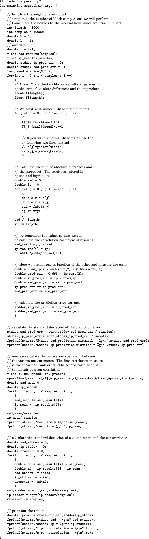
and gasdev from [17].
In all cases, both
the linear Pearson and spearman rank order correlations were similar.
The programs to measure the correlations can be found in section
appendix.
and then from a normal distribution. The random generators are ran2
and gasdev from [17].
In all cases, both
the linear Pearson and spearman rank order correlations were similar.
The programs to measure the correlations can be found in section
appendix.
|
||||||||||||||||||||||||||||||||||||||||||||||||||||||||||||||||||||||||||||||||||||||||||||||||||||||||
3 Correlation estimate between the inproduct and the sum of absolute differences
We now assume that both vectors ![]() and
and ![]() are uniform distributed
within range
are uniform distributed
within range ![]() , with
, with ![]() and
and ![]() .
. ![]() denotes the size
of the interval (
denotes the size
of the interval (![]() ). The comparators
). The comparators ![]() and
and
![]() ,
both depending on
,
both depending on ![]() and
and ![]() , will now be considered to be variables
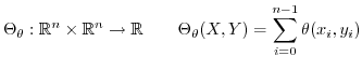
themselves. The correlation between them,
, will now be considered to be variables
themselves. The correlation between them,
![]() ,
is given by
,
is given by
![$\displaystyle \frac{\mathbb{E}[\Theta_{\times}.\Theta_{\left\vert-\right\vert}]...
...{\left\vert-\right\vert}^{2}]-\mathbb{E}[\Theta_{\left\vert-\right\vert}]^{2}}}$](img109.png) |
(7) |
Under the assumption that the various sample positions are independent
from each other, one can easily show that
![]() .
.
![$\displaystyle \frac{\mathbb{E}[\theta_{\times}\theta_{\left\vert-\right\vert}]-...
...{\left\vert-\right\vert}^{2}]-\mathbb{E}[\theta_{\left\vert-\right\vert}]^{2}}}$](img111.png)
This reduces the 5 estimates we need to
![]() ,
, ![]() ,
,
![]() ,
,
![]() and
and
![]() . We will now determine those
5 values.
. We will now determine those
5 values.
3.1 Estimate of 
Estimates of a variable ![]() can be calculated from probability functions
as follows (
can be calculated from probability functions
as follows (![]() is the
probability distribution function of the variable
is the
probability distribution function of the variable
![]() )
)
![$\displaystyle \mathbb{E}[T]=\int_{-\infty}^{+\infty}x.p(x)dx$](img119.png)
To calculate the probability distribution function of ![]() with
both
with
both ![]() and
and ![]() uniform distributions over
uniform distributions over ![]() , we must first
obtain the probability function of
, we must first
obtain the probability function of ![]() , which is given by [18]:
, which is given by [18]:
![$\displaystyle _{x-y}(u)=\begin{cases}
\frac{t-u}{t^{2}} & \mbox{for }u\in[0,t]\\
\frac{t+u}{t^{2}} & \mbox{for }u\in[-t,0]\end{cases}$](img121.png)
Since this probability distribution is symmetrical around ![]() (the
means of the two uniform distribution has been subtracted), we would
get an expected value of 0, but then we would forget to take into
account the absolute difference. englishThe absolute
difference will flip the probability of all values below zero over
the vertical axis and add them there. This will result in an increased
slope to the right and a probability density of 0 for negative values
[19].
(the
means of the two uniform distribution has been subtracted), we would
get an expected value of 0, but then we would forget to take into
account the absolute difference. englishThe absolute
difference will flip the probability of all values below zero over
the vertical axis and add them there. This will result in an increased
slope to the right and a probability density of 0 for negative values
[19].
![\includegraphics[width=0.5\textwidth]{pdfad}](img123.png)
![$\displaystyle _{\vert x-y\vert}(u)=\begin{cases}2\frac{t-u}{t^{2}} & \mbox{for }u\in[0,t]\\ 0 & \mbox{otherwise}\end{cases}$](img124.png)
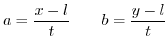
Figure 1 plots eq.8. englishThe expectancy can now be calculated
![$\displaystyle \mathbb{E}[\left\vert x-y\right\vert]=\int_{0}^{h-l}2u\frac{t-u}{t^{2}}du=\frac{t}{3}$](img125.png) |
(9) |
Testing this empirically gives the following values:
![]() ,
,
![]() ,
,
![]() ,
,
![]() ,
,
![]() and
and
![]() . Which is consistent
to the above formula.
. Which is consistent
to the above formula.
3.2 Estimate of 
![$\displaystyle \mathbb{E}[g(x)]=\int_{-\infty}^{+\infty}g(x)f(x)dx$](img133.png) |
(10) |
we can calculate ![]() based on the previous probability
density function (8) as
based on the previous probability
density function (8) as
![$\displaystyle \mathbb{E}[\vert x-y\vert^{2}]=\int_{0}^{h-l}2u^{2}\frac{t-u}{t^{2}}du=\frac{t^{2}}{6}$](img135.png) |
(11) |
Testing this empirically gives the following values:
![]() ,
,
![]() ,
,
![]() ,
,
![]() ,
,
![]() and
and
![]() . Which is
close to the results as given by eq. 11.
. Which is
close to the results as given by eq. 11.
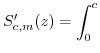
3.3 Estimate of 
To determine ![]() we will calculate the probability
distribution function of
we will calculate the probability
distribution function of ![]() , which might appear as taking the
long road when the probability distribution of uniform products on
, which might appear as taking the
long road when the probability distribution of uniform products on
![]() is already known [20]. However, we will
later on needs this probability distribution on
is already known [20]. However, we will
later on needs this probability distribution on ![]() to determine
to determine
![]() and
and
![]() and
we can now introduce the technique we will also use in section 3.5.2.
and
we can now introduce the technique we will also use in section 3.5.2.
The probability
density function of ![]() is defined as
the differential
of the cumulative probability function, which in turn is defined as
is defined as
the differential
of the cumulative probability function, which in turn is defined as
|
![\includegraphics[width=0.3\textwidth]{xyz1}](img145.png)
![\includegraphics[width=0.3\textwidth]{xyz2}](img146.png)
![\includegraphics[width=0.3\textwidth]{xyz3}](img147.png)
Figure 2 illustrates how to find the number of
values
(of ![]() ) located below a fixed
) located below a fixed ![]() . The surface area that is not
cut off at
. The surface area that is not
cut off at ![]() directly
reflects the probability that a value below
directly
reflects the probability that a value below
![]() can be chosen because both
can be chosen because both ![]() and
and ![]() are uniformly distributed.
Since the isoline of
are uniformly distributed.
Since the isoline of ![]() is
located at
is
located at ![]() , various
forms of
, various
forms of ![]() can be combined.
can be combined.
![]() suffers from a discontinuity at 0 when
suffers from a discontinuity at 0 when ![]() and its calculation
in this particular context is further complicated with a sudden
quadrant-change
of the isoline when
and its calculation
in this particular context is further complicated with a sudden
quadrant-change
of the isoline when ![]() becomes
negative. In which case quadrant
1 and 3 no longer contain the isoline. Instead, quadrant 2 and 4 will
contain it (see figure 3 for an
illustration). To
approach this problem, we divided the calculation of
CDF
becomes
negative. In which case quadrant
1 and 3 no longer contain the isoline. Instead, quadrant 2 and 4 will
contain it (see figure 3 for an
illustration). To
approach this problem, we divided the calculation of
CDF![]() into three branches. The first with
into three branches. The first with ![]() ; The second with
; The second with ![]() and the last with
and the last with ![]() .
.
|
![\includegraphics[width=0.5\textwidth]{xy1}](img154.png)
![\includegraphics[width=0.5\textwidth]{xy2}](img155.png)
Aside from these standard complications, we must also limit our ![]() and
and ![]() values to the range
values to the range ![]() . This restricts the maximal
surface area we can find and requires a piecewice approach. We start
out with a general solutions for rectangles originating in
. This restricts the maximal
surface area we can find and requires a piecewice approach. We start
out with a general solutions for rectangles originating in
![]() and ending at a specific point. We have the following 4 sections:
and ending at a specific point. We have the following 4 sections:
![\begin{displaymath}
\begin{array}{cc}
S_{1}:\, x,y\in[0:h,0:h] & S_{2}:\, x,y\in...
...
S_{3}:\, x,y\in[0:l,0:l] & S_{4}:\, x,y\in[0:h,0:l]\end{array}\end{displaymath}](img157.png)
![\includegraphics[width=0.5\textwidth]{sections}](img158.png)
Every section forms the two dimensional bounds (on ![]() and
and ![]() )
for the integral
)
for the integral ![]() , and depending on the sign of
, and depending on the sign of
![]() they wil be added or
substracted to/from each other. Figure
4 presents this graphically. When
they wil be added or
substracted to/from each other. Figure
4 presents this graphically. When ![]() is positive
we need to subtract
is positive
we need to subtract ![]() and
and ![]() , otherwise we need to add
them.
, otherwise we need to add
them. ![]() is used to
denoted the size of area
is used to
denoted the size of area ![]() intersected
with the area below the isoline. The cumulative distribution function
is now defined as
intersected
with the area below the isoline. The cumulative distribution function
is now defined as
CDF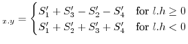 |
(12) |
 min
min![\includegraphics[width=0.5\textwidth]{xyclip}](img171.png)
![]() can be
determined by first obtaining the x-point where
the hyperbole crosses the top line of our box, which happens at
position
can be
determined by first obtaining the x-point where
the hyperbole crosses the top line of our box, which happens at
position
![]() .
When
.
When ![]() and
and ![]() are positive, this point will
always be larger than 0. When
are positive, this point will
always be larger than 0. When ![]() , the intersection will happen
outside
, the intersection will happen
outside ![]() , in which case the surface area will be
, in which case the surface area will be ![]() . When
. When
![]() we need to integrate
we need to integrate
![]() and
and
![]() (See figure 5 for an illustration), which gives
(See figure 5 for an illustration), which gives
 |
(14) |
3.3.1 Cumulative
probability when  is positive
The cumulative probability function (13)
requires
us to calculate the different sections based on (14)
with ![]() ;
; ![]() and
and ![]() .
Since (14) appears to be discontinue at
position
.
Since (14) appears to be discontinue at
position
![]() we split the cumulative
probability function in 4 segments.
we split the cumulative
probability function in 4 segments.
When ![]() the cumulative probability
is 0 because there can
be no values
the cumulative probability
is 0 because there can
be no values ![]() and
and ![]() , both larger than
, both larger than ![]() that can lead
to
a multiple that is smaller than
that can lead
to
a multiple that is smaller than ![]() .
.
| CDF |
 ln ln |
||
| (15) |
| CDF |
(17) |
![\includegraphics[width=0.36\textwidth]{pdfxylhpos}](img206.png)
![\includegraphics[width=0.64\textwidth]{pdfxylhneg}](img207.png)
(15), (16) and (17)
are the non-normalized
cumulative distribution functions americanwhen
![]() . Given the maximum surface
area (17), we can divide
and differentiate them all to provide us with the proper probability
distribution (illustrated in figure 6).
We
conclude that, when
. Given the maximum surface
area (17), we can divide
and differentiate them all to provide us with the proper probability
distribution (illustrated in figure 6).
We
conclude that, when ![]() :
:
![$\displaystyle _{x.y}(z)=\begin{cases}\frac{\mbox{ln}z-2\mbox{ln}l}{t^{2}} & \mb...
...mbox{ln}z}{t^{2}} & \mbox{for }z\in[lh,h^{2}]\\ 0 & \mbox{otherwise}\end{cases}$](img208.png)
3.3.2 Cumulative
probability when  is negative
When ![]() the result is somewhat more complex.
Instead
of subtracting
the result is somewhat more complex.
Instead
of subtracting ![]() , we need to add them. The interesting thing
is that neither
, we need to add them. The interesting thing
is that neither ![]() nor
nor ![]() will intersect with
will intersect with ![]() ,
when
,
when ![]() . However, as soon as
. However, as soon as ![]() the situation is different.
(depicted in fig. 3). Therefore we further
branch
the calculation.
the situation is different.
(depicted in fig. 3). Therefore we further
branch
the calculation.
3.3.2.1 z>0
When ![]() we have
we have ![]() as surface area for
as surface area for ![]() and
and ![]() .
.
| (19) |
![$\displaystyle S'_{1}(z)=\begin{cases}z(1+2\mbox{ln}h-\mbox{ln}z) & \mbox{for }z\in[0,h²]\\ h^{2} & \mbox{for }z>h^{2}\end{cases}$](img216.png)
![$\displaystyle S'_{3}(z)=\begin{cases}z(1+2\mbox{ln}(-l)-\mbox{ln}z) & \mbox{for }z\in[0,l²]\\ l² & \mbox{for }z>l^{2}\end{cases}$](img218.png)
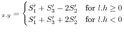
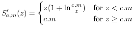
3.3.2.2 z<0
When ![]() we are
interested in the outside of the function
we are
interested in the outside of the function ![]() ,
which is to be found in
,
which is to be found in ![]() and
and ![]() . Since the area below
the curve matches that as if
. Since the area below
the curve matches that as if ![]() ,
, ![]() and
and ![]() were positive, we
get surface area
were positive, we
get surface area ![]() (The minus signs have been added to make
(The minus signs have been added to make ![]() and
and ![]() positive). As such, the remaining surface area must then be
positive). As such, the remaining surface area must then be
![$\displaystyle S'_{2,4}(z)=\begin{cases}-l.h+z(1+ln\frac{lh}{z}) & \mbox{for }z\in[lh,0]\\ -l.h & \mbox{for }z<l.h\end{cases}$](img221.png) |
(22) |
![$\displaystyle _{x.y}(z)=\begin{cases}-2lh & z<l.h\\ 2(-lh+z(1+\mbox{ln}\frac{l....
...+\mbox{ln}\frac{h^{2}}{z}) & z\in[l^{2},h^{2}]\\ l²-2lh+h² & z>h^{2}\end{cases}$](img224.png)
![$\displaystyle _{x.y}(z)=\begin{cases}\frac{2\mbox{ln}h+2\mbox{ln}l-2\mbox{ln}z}...
...x{ln}h-\mbox{ln}z}{t^{2}} & z\in[l^{2},h^{2}]\\ 0 & \mbox{otherwise}\end{cases}$](img226.png)
3.3.3 The estimate of
The estimate of ![]() is calculated
as
is calculated
as
![$\displaystyle \mathbb{E}[x.y]=\int_{-\infty}^{+\infty}z.$](img229.png) PDF
PDF3.3.3.1 when 

3.3.3.2 when 
Since (28)==(29)
we have in the
general case:
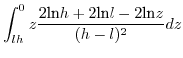
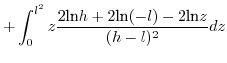
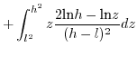
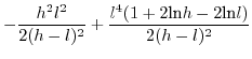
![$\displaystyle \mathbb{E}[x.y]=\left(\frac{h+l}{2}\right)^{2}$](img240.png)
3.4 Estimate of

The probability density function of ![]() is given in (18)
and (25).
is given in (18)
and (25).
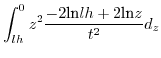
3.4.1 When 
![$\displaystyle \int_{l^{2}}^{h^{2}}\frac{z^{2}}{t^{2}}\begin{cases}
ln\frac{z}{l^{2}} & z\in[l^{2},lh]\\
ln\frac{h²}{z} & z\in[lh,h^{2}]\end{cases}d_{z}$](img242.png)

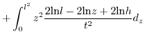
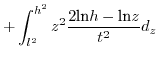
3.4.2 When 
The situation when ![]() is discussed below. We first start with
the case where
is discussed below. We first start with
the case where ![]() . This gives us
. This gives us
![$\displaystyle \int_{l.h}^{h^{2}}2\frac{z^{2}}{t^{2}}\begin{cases}
ln\frac{z}{l....
...ac{l.h}{z} & z\in[0,l^{2}]\\
ln\frac{l}{z} & z\in[l^{2},h^{2}]\end{cases}d_{z}$](img247.png)
Since (31)==(32), we conclude that
![$\displaystyle \mathbb{E}\left[(x.y)^{2}\right]=\left(\frac{h^{3}-l^{3}}{3t}\right)^{2}$](img252.png) |
(33) |
3.5 Estimate of

If we define ![]() and
and ![]() to be the translation and scaling of
to be the translation and scaling of ![]() and
and ![]() as follows
as follows
then ![]() and
and ![]() are uniform distributed over
are uniform distributed over ![]() . americanThe
variable
. americanThe
variable ![]() (and
(and ![]() ) can also be defined in function of
) can also be defined in function of ![]() as
as
| (34) |
This substitution will make it possible to rewrite
![]()
| (35) |
3.5.1 Estimating
![$ \mathbb{E}[a\vert a-b\vert]$](img275.png)
![]() becomes
becomes
![]() and
and ![]() are uniform distributions, as such
are uniform distributions, as such
![]() .
The estimates for
.
The estimates for ![]() (under
condition that
(under
condition that ![]() ) and
) and ![]() (under condition that
(under condition that ![]() will be the same:
will be the same:
![$\displaystyle \mathbb{E}[a.b\vert a>b]=\int_{0}^{1}-z$](img282.png) ln ln |
(36) |
Without the condition that ![]() we need to double the estimate of
(36)
we need to double the estimate of
(36)
![$\displaystyle \mathbb{E}[a\vert a-b\vert]=2(\frac{1}{3}-\frac{1}{4})=\frac{1}{6}$](img284.png)
(35) becomes
![$\displaystyle \mathbb{E}\left[x.y\left\vert x-y\right\vert\right]=t³\mathbb{E}[a.b.\vert a-b\vert]+\frac{t^{2}l+tl^{2}}{3}$](img285.png) |
(37) |
3.5.2 Estimating
![$ \mathbb{E}[a.b.\vert a-b\vert]$](img286.png)
The factors ![]() and
and ![]() are not
independent, therefore we
cannot rely on the standard rule for uniform products [20].
In order to resolve this we divide the space of possible values in
those which
are not
independent, therefore we
cannot rely on the standard rule for uniform products [20].
In order to resolve this we divide the space of possible values in
those which ![]() and those
with
and those
with ![]() . This gives, due to linearity
of
. This gives, due to linearity
of ![]() the following:
the following:
![$\displaystyle \mathbb{E}[a.b\vert a-b\vert]=\begin{cases}\mathbb{E}[a²b]-\mathb...
... & \mbox{for }a>b\\ \mathbb{E}[ab²]-\mathbb{E}[a²b] & \mbox{for }b>a\end{cases}$](img290.png) |
(38) |
![\includegraphics[width=0.3\textwidth]{xxy3d1}](img293.png)
![\includegraphics[width=0.3\textwidth]{xxy3d2}](img294.png)
![\includegraphics[width=0.3\textwidth]{xxy3d3}](img295.png)
Plotting ![]() (figure 7) reveals the areas
that we are interested in. The plots have been clipped at a specific
value of
(figure 7) reveals the areas
that we are interested in. The plots have been clipped at a specific
value of ![]() . All positions where
. All positions where ![]() was larger than
was larger than ![]() have been removed. So, the surface area of the plots that is not
clipped
forms the cumulative probability that a specific combination of
have been removed. So, the surface area of the plots that is not
clipped
forms the cumulative probability that a specific combination of ![]() will be lower than
will be lower than ![]() . Of course, we are not only interested in
understanding the size of the area, but we also need to take into
account the extra condition that
. Of course, we are not only interested in
understanding the size of the area, but we also need to take into
account the extra condition that ![]() .
.
![\includegraphics[width=0.49\textwidth]{xxyisoline}](img296.png)
|
![\includegraphics[width=0.49\textwidth]{xxyisoline2}](img297.png) |
For a fixed value of ![]() we
can calculate the isoline as (taking
into account that
we
can calculate the isoline as (taking
into account that ![]() ) min
) min![]() . Figure
8 presents the shape of this function.
The surface
area under this curve is the area where
. Figure
8 presents the shape of this function.
The surface
area under this curve is the area where ![]() while still respecting
that
while still respecting
that ![]() . Integrating this equation provides us with the cumulative
distribution function (39). To do so, we need
to know
where the linear 45 degree line cuts the function
. Integrating this equation provides us with the cumulative
distribution function (39). To do so, we need
to know
where the linear 45 degree line cuts the function
![]() .
.
| (40) |
This now allows us to write down the surface area below as a couple of integrals
| CDF |
![$\displaystyle \int_{0}^{\sqrt[3]{z}}ada+\int_{\sqrt[3]{z}}^{1}\frac{z}{a^{2}}da$](img304.png) |
||
 |
![\includegraphics[width=0.5\textwidth]{pdfaab1}](img306.png)
|
![\includegraphics[width=0.5\textwidth]{pdfaab2}](img307.png) |
This function has a maximum of 0.5 at 1, so we need to multiply it
by two to get a proper cumulative distribution function.
Differentiating
it afterward gives the probability density function of ![]() (left
as calculated; right by sapping variables
(left
as calculated; right by sapping variables ![]() and
and ![]() ). Figure 9a
plots (41).
). Figure 9a
plots (41).
![\begin{displaymath}\begin{array}{l} \mbox{PDF}_{a^{2}b\vert b<a}(z)=\frac{2}{\sq...
...ox{PDF}_{b^{2}a\vert a<b}(z)=\frac{2}{\sqrt[3]{z}}-2\end{array}\end{displaymath}](img309.png) |
(41) |
Since we cannot rely on a symmetry around the 45 degree angle, we
also need to calculate the surface area when ![]() . The isoline is
given as min
. The isoline is
given as min![]() max
max![]() . Figure 8
provides more insight in the shape of this function. The function
appears piecewise, with first a constant line (1) and then a hyperbolic
piece up to its crossing with the 45 degree slope. Under these two
segments we also have a linear piece that we need to subtract from
the volume. For a fixed
. Figure 8
provides more insight in the shape of this function. The function
appears piecewise, with first a constant line (1) and then a hyperbolic
piece up to its crossing with the 45 degree slope. Under these two
segments we also have a linear piece that we need to subtract from
the volume. For a fixed ![]() we
determine the crossing of 1 with
we
determine the crossing of 1 with ![]() and the crossing between
and the crossing between ![]() and
and ![]() . The first
crossing occurs at position
. The first
crossing occurs at position ![]() . The second crossing occurs
at
. The second crossing occurs
at ![]() (40).
(40).
We can now calculate the surface area as
| CDF |
![$\displaystyle \int_{0}^{\sqrt{z}}1da+\int_{\sqrt{z}}^{\sqrt[3]{z}}\frac{z}{a^{2}}da$](img316.png) |
||
![$\displaystyle -\int_{0}^{\sqrt[3]{z}}ada$](img317.png) |
(42) | ||
| (43) |
![\begin{displaymath}\begin{array}{l} \mbox{PDF}_{a^{2}b\vert b>a}(z)=\frac{2}{\sq...
...ert a>b}(z)=\frac{2}{\sqrt{z}}-\frac{2}{\sqrt[3]{z}}\end{array}\end{displaymath}](img320.png)
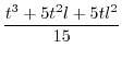
Combining (41) and (44) leads
to the following
estimates for ![]() (38)
(38)
![$\displaystyle \int_{0}^{1}z.(\frac{2}{\sqrt[3]{z}}-2)dz$](img324.png) |
|||
![$\displaystyle \int_{0}^{1}z(\frac{2}{\sqrt{z}}-\frac{2}{\sqrt[3]{z}})dz$](img328.png) |
|||
![$\displaystyle \mathbb{E}[a.b\vert a-b\vert]=\left\{ \begin{array}{cc}
\mathbb{E...
...] & a>b\\
\mathbb{E}[ab²]-\mathbb{E}[a²b] & b>a\end{array}\right.=\frac{1}{15}$](img330.png)
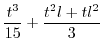
3.5.3 Estimating 
Knowing the value for ![]()
![]() makes
it possible to finish (37) :
makes
it possible to finish (37) :
 |
|||
 |
(45) |
Testing this empirically gives the following values:
![]() ,
,
![]() ,
,
![]() ,
,
![]() ,
,
![]() ,
,
![]() and
and
![]() .
Which is correct with the above formula.
.
Which is correct with the above formula.
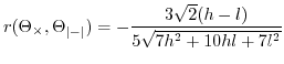
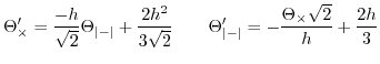
3.6 The Correlation Coëfficient
The correlation coefficient between ![]() and
and
![]() (7) is given as:
(7) is given as:
![$\displaystyle r(\Theta_{\times},\Theta_{\left\vert-\right\vert})=\frac{\mathbb{...
...rt x-y\vert]}{\sigma_{\theta_{\times}}\sigma_{\theta_{\left\vert-\right\vert}}}$](img343.png) |
(46) |
![\includegraphics[width=0.5\textwidth]{correlationplot}](img350.png)
|
Figure fig:correlationipadplot shows the correlation strength
in function of ![]() and
and ![]() . Surprisingly the correlation for any
point with
. Surprisingly the correlation for any
point with ![]() is
is
![]() . The
maximal correlation is found with
. The
maximal correlation is found with ![]() , which is then
, which is then
 for for |
(47) |
4
Estimating  in function
of
in function
of  and vice versa
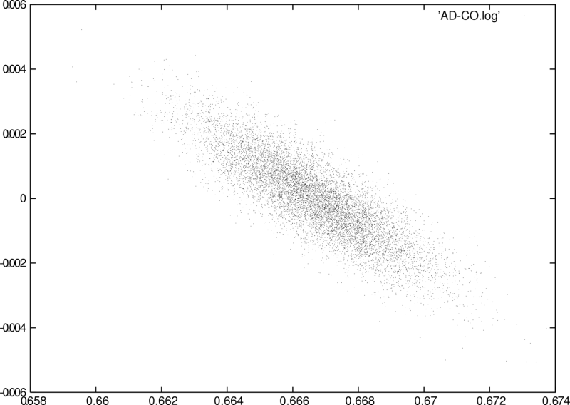
Figure 11 illustrates the
correlation
between ![]() and
and
![]() with
with ![]() .
Since every block comparison is the summation of variables of the
same distribution we get in the end a Gaussian distribution [21]with means equal to the means of the underlying operators
.
Since every block comparison is the summation of variables of the
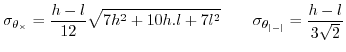
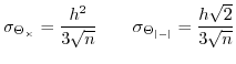
same distribution we get in the end a Gaussian distribution [21]with means equal to the means of the underlying operators ![]() and a standard deviation that should be divided by
and a standard deviation that should be divided by ![]() . The
standard deviations of
. The
standard deviations of ![]() and
and ![]() are
are
Which means that following the central limit theorem [21],
we get, when ![]() , the following standard deviations for the block
operators
, the following standard deviations for the block
operators ![]() and
and
![]() .
.
 |
(48) |
![$\displaystyle \frac{\Theta_{\times}-\mathbb{E}\left[\Theta_{\times}\right]}{\si...
...heta_{\left\vert-\right\vert}\right]}{\sigma_{\Theta_{\left\vert-\right\vert}}}$](img360.png)
Taking out ![]() allows us to predict it based on the
measurement of
allows us to predict it based on the
measurement of ![]() . We call the predictions
respectively
. We call the predictions
respectively ![]() and
and
![]() .
.
| (49) |
The expected difference between ![]() and
and
![]() is 0 as shown below:
is 0 as shown below:
![$\displaystyle \mathbb{E}\left[-\frac{\left(\Theta_{\left\vert-\right\vert}-\mat...
...rt-\right\vert}}}+\mathbb{E}\left[\Theta_{\times}\right]-\Theta_{\times}\right]$](img368.png) |
|||
| (51) | |||
| (52) | |||
| 0 | (53) |
(54) can be deduced as follows:
![$\displaystyle \sigma_{a'-a}=\sqrt{\mathbb{E}\left[\left(a'-a\right)^{2}\right]-\mathbb{E}\left[a'-a\right]^{2}}$](img376.png)
Since the second term is known to be zero (53), we have
| (55) | |||
| (56) |
![$\displaystyle \mathbb{E}\left[\left(-\frac{\left(b-\mathbb{E}\left[b\right]\right)\sigma_{a}}{\sigma_{b}}+\mathbb{E}\left[a\right]\right)^{2}\right]$](img383.png) |
|||
![$\displaystyle \frac{\sigma_{a}^{2}}{\sigma_{b}^{2}}\mathbb{E}\left[\left(b-\mathbb{E}\left[b\right]\right)^{2}\right]$](img384.png) |
|||
![$\displaystyle -2\frac{\sigma_{a}\mathbb{E}\left[a\right]}{\sigma_{b}}\mathbb{E}\left[b-\mathbb{E}\left[b\right]\right]+\mathbb{E}\left[a\right]^{2}$](img385.png) |
|||
| (57) |
![$\displaystyle \mathbb{E}\left[-\frac{\left(b-\mathbb{E}\left[b\right]\right)\sigma_{a}a}{\sigma_{b}}+a\mathbb{E}\left[a\right]\right]$](img389.png)
![$\displaystyle r_{a,b}=\frac{\mathbb{E}\left[ab\right]-\mathbb{E}\left[a\right]\mathbb{E}\left[b\right]}{\sigma_{a}\sigma_{b}}$](img392.png)
we have that
![]() and thus (58) becomes
and thus (58) becomes
| (59) |
with ![]() this becomes
this becomes
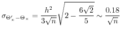
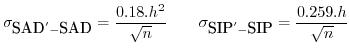
Both are interesting because they allow us to determine a confidence interval for the estimation based on the block size.
For a length ![]() we get a standard deviation
of the prediction
error of the
we get a standard deviation
of the prediction
error of the ![]() -mismatch as
-mismatch as ![]() . If we
would work on the interval
. If we
would work on the interval ![]() , we would get
a prediction mismatch of
, we would get
a prediction mismatch of ![]() . On the interval
. On the interval ![]() ,
the prediction mismatch would be
,
the prediction mismatch would be ![]() . This seems large but
the expected results for
. This seems large but
the expected results for ![]() are large as
well if we
work with
are large as
well if we
work with ![]() . For length
. For length ![]() ,
, ![]() we get a standard
deviation of
we get a standard
deviation of ![]() . For a length of
. For a length of ![]() we have a standard
deviation of
we have a standard
deviation of ![]() . The standard deviation of the
. The standard deviation of the ![]() prediction based on
prediction based on ![]() for length
for length ![]() is
is ![]() .
For
.
For ![]() this becomes
this becomes
![]() and
and ![]() gives
gives
![]() .
.
5 Discussion
5.1 Bias and non-correlation
It is easy to recognize that a baseline added to any of the two comparator blocks, will not influence the correlation value, it will merely increase the variance of the inproduct, while it will increase the value of the SAD. This results in predictions that might be 'off by a baseline'. Therefore, when using this technique in a sliding window setup, one might consider appropriate techniques to remove baselines, such as low pass filtering, multirate signal processing and so on [12, 17].
A second observation of importance is that zeros, in either block, will influence the reliability of the correlation. The more zeros, the more the SAD and the inproduct will differ. The inproduct essentially skips zeros and always returns a 'minimal match', irrelevant of the other value. The absolute difference will not be influenced by zeros, and will treat them as any other value, and thus still distinguish properly.
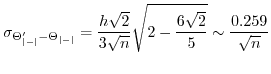
5.2 Auto-Comparison
As a practical application we investigated the similarity between
auto-correlation and the lagging sum of absolute differences,
respectively
defined as ![]() and
and ![]() :
:
|
The input dataset were the first ![]() samples of a song, which
were then equalized and scaled to the range
samples of a song, which
were then equalized and scaled to the range
![]() .
On this dataset we calculated
.
On this dataset we calculated ![]() and
and ![]() , plotted in figure 12
in red and green respectively. The predicted values of
, plotted in figure 12
in red and green respectively. The predicted values of ![]() and
and ![]() in function of the other are respectively purple and blue. We find
that the predictions are fairly accurate and allow the recognition
of the same peaks as one goes along. Near the end of the dataset
in function of the other are respectively purple and blue. We find
that the predictions are fairly accurate and allow the recognition
of the same peaks as one goes along. Near the end of the dataset ![]() appears biased due to the window size, which becomes smaller as the
lag increases.
appears biased due to the window size, which becomes smaller as the
lag increases. ![]() reflects this
in its variance. The similarity
between
reflects this
in its variance. The similarity
between ![]() and
and ![]() has already led to an application in
meta data
extraction, in which an algorithmic approach, using the SAD, assesses
music-tempo slightly faster and with less memory requirements than
conventional auto-correlation. This has been implemented in the
DJ-program BpmDj [22, 23].
has already led to an application in
meta data
extraction, in which an algorithmic approach, using the SAD, assesses
music-tempo slightly faster and with less memory requirements than
conventional auto-correlation. This has been implemented in the
DJ-program BpmDj [22, 23].
5.3 Block Matching
|
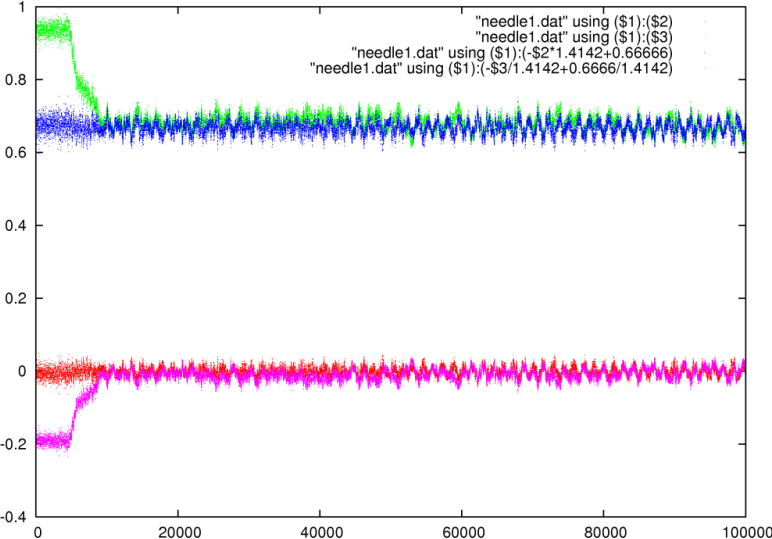
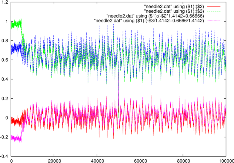
A second test we conducted was finding a pattern (called the needle)
in a larger data set (the haystack). As a haystack we used the first
![]() equalized
samples of a song. We generated two needles.
The first one was a random white noise pattern, the second one was
a random block taken from the haystack. Both needles were
equalized
samples of a song. We generated two needles.
The first one was a random white noise pattern, the second one was
a random block taken from the haystack. Both needles were ![]() samples long. Using a sliding window block comparator we plotted the
inproduct and the SAD, as well as their predicted values (Figure 13).
As observed before, when the inproduct increases, the sad decreases
and vice versa. Both plots start with an unexpected large sad and
noisy inproduct because the song starts with some ambiance, which
are many values near zero. Therefore in this area, the inproduct had
a smaller variance than the rest of the song while the sad was larger
than expected. The needle we looked for in the second test was taken
from the middle of the haystack. At this position we indeed find a
peaking of all values.
samples long. Using a sliding window block comparator we plotted the
inproduct and the SAD, as well as their predicted values (Figure 13).
As observed before, when the inproduct increases, the sad decreases
and vice versa. Both plots start with an unexpected large sad and
noisy inproduct because the song starts with some ambiance, which
are many values near zero. Therefore in this area, the inproduct had
a smaller variance than the rest of the song while the sad was larger
than expected. The needle we looked for in the second test was taken
from the middle of the haystack. At this position we indeed find a
peaking of all values.
5.4 Local matching
In auto-comparison and block searching we find the same peaks back and, skipping the baseline, at a local level the inproduct behaves similar to the SAD. This makes clear that whatever technique one uses to find a global match, both the inproduct and SAD are equally valid to find local minima. This has an important application in landmark tracking, which can be done equally well with Fourier transformations as with the widely used SAD.
5.5 Equalization of the amplitudes
The equalization of amplitudes can be easily conducted for sound waves
or color images. There one simply counts the number of occurrences
of specific amplitudes, which is an
![]() operation.
Afterwards , a cumulative distribution of this binned histogram can
be made. The total cumulative value can then form the divisor for
all the binned numbers.
operation.
Afterwards , a cumulative distribution of this binned histogram can
be made. The total cumulative value can then form the divisor for
all the binned numbers.
If ![]() is the number of time the
value
is the number of time the
value ![]() occurred in
the audio-stream,
then we define
occurred in
the audio-stream,
then we define ![]() as
as
![$\displaystyle C[v]=\sum_{i=0}^{v}B[i]$](img426.png)
The maximal value is found at ![]() . (
. (![]() standing for maximum
amplitude). The equalization of the histogram now consists of assigning
a floating point value to each of the original inputs and using those
values. The lookup table will be called
standing for maximum
amplitude). The equalization of the histogram now consists of assigning
a floating point value to each of the original inputs and using those
values. The lookup table will be called ![]()
![$\displaystyle M[v]=\frac{2.C[v]}{C[m]}-1$](img429.png)
Translating the original signal through ![]() will make it uniform
distributed as
will make it uniform
distributed as
This operation is ![]() . It has however some
memory lookups that might be unattractive for long sequences. The
next question is whether on real signals, how well the correlation
holds. Can we for instance find the
. It has however some
memory lookups that might be unattractive for long sequences. The
next question is whether on real signals, how well the correlation
holds. Can we for instance find the
6 Summary
If two data sequences are uniformly sampled from -1:1 then both the summed inproduct (SIP) and the sum of absolute differences (SAD) behave similarly, with a correlation coefficient of -0.8485. This useful relationship allows the prediction of one operator in function of the other as follows:
SIP SAD SAD |
SAD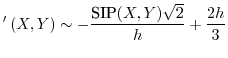 |
Applications of this relation might, among others, include optimizations in the areas of sound analysis, pattern-matching, digital image processing and compression algorithms (such as rsync).
The use of absolute difference was attractive because it offers a way to compare signals such that mismatches could not cancel each other out thereby providing the same result independent of any constant added to the signal. Convolution did not behave as such and in fact provided, in our view, not the best manner of comparing two signals: it was dependent on the constant added to the signal (which can happen due to very low frequency oscillation that cannot be captured in the window). On the other hand, when many comparisons are necessary, the inproduct can be implemented very efficiently by means of Fourier transformation.
Regarding the proof and formulas used in this document: it is probably the worst piece of math I've ever been involved with. It is tedious, complicated and at the moment I have no clue how I could simplify it. Probably there are some black magic tricks mathematicians could use, but not being a native mathematician, I'm stuck with what I have.
Bibliography
| 1. | Building Blocks for MPEG Stream Processing Stephan Wong, Jack Kester, Michiel Konstapel, Ricardo Serra, Otto Visser institution: Computer Engineering Laboratory, Electrical Engineering Department, Delft University of Technology; 2002 |
| 2. | Fast Sum of Absolute Differences Visual Landmark Detector Craig Watman, David Austin, Nick Barnes, Gary Overett, Simon Thompson Proceedings of IEEE Conference on Robotics and Automation; April; 2004 |
| 3. | The Sum-Absolute-Difference Motion Estimation Accelerator S. Vassiliadis, E.A. Hakkennes, J.S.S.M. Wong, G.G. Pechanek EUROMICRO 98 Proceedings of the 24th EUROMICRO Conference, Vasteras, Sweden, pp. 559-566, Aug 1998, IEEE Computer Society, ISBN: 0-8186-8646-4.; 1998 |
| 4. | Real-time Area Correlation Tracker Implementation based on Absolute Difference Algorithm Weichao Zhou, Zenhan Jiang, Mei Li, Chunhong Wang, Changhui Rao Optical Engineering; volume: 42; number: 9; pages: 2755-2760; September; 2003 |
| 5. | Employing Difference Image in Affine Tracking G. Jing, D. Rajan, C.E.Siong Signal and Image Processing; 2006 |
| 6. | Absolute Difference Generator for use in Display Systems David F. McManigal howpublished: United States Patent 4218751; March 7; 1979 |
| 7. | Arithmetic circuit for calculating the absolute value of the difference between a pair of input signals Masaaki Yasumoto, Tadayoshi Enomoto, Masakazu Yamashina howpublished: United States Patent 4,849,921; June; 1989 |
| 8. | Calculating the absolute difference of two integer numbers in a single instruction cycle Roney S. Wong howpublished: United States Patent 5835389; April; 1996 |
| 9. | Adaptive Bit-Reduce Mean Absolute Difference criterion for block-matchin algorithm and its VLSI Design Hwang-Seok Oh, Yunju Baek, Heung-Kyu Lee Opt. Eng.; volume: 37; number: 12; pages: 3272-3281; December; 1998 |
| 10. | Numerical Recipes in C++ William T. Veterling, Brian P. Flannery Cambridge University Press; editor: William H. Press and Saul A. Teukolsky; chapter: 15.7; edition: 2nd; February; 2002 |
| 11. | Do Aligned Sequences Share the Same Fold ? Ruben A. Abagyan, Serge Batalov Journal of Molecular Biology; 1997 |
| 12. | Discrete-Time Signal Processing Alan V. Oppenheim, Ronald W. Schafer Prentice Hall; editor: John R. Buck; 1989 |
| 13. | Juggling with Pattern Matching Jean Cardinal, Steve Kremer, Stefan Langerman institution: Universite Libre De Bruxelles; 2005 |
| 14. | A Randomized Algorithm for Approximate String Matches Mikhail J. Atallah, Frederic Chyzak, Philippe Dumas Algorithmica; volume: 29; number: 3; pages: 468-486; 2001 |
| 15. | Scientific Visualization: The Visual Extraction of Knowledge from Data Julia Ebling, Gerik Scheuermann Berlin Springer; editor: G.P. Bonneau and T. Ertl and G.M. Nielson; chapter: Clifford Convolution And Pattern Matching On Irregular Grids; pages: 231-248; 2005 |
| 16. | The Art of Computer Programming Donald Knuth Addison-Wesley; chapter: 1.2.11: Asymptotic Representations; pages: 107-123; volume: 1; edition: 3th; 1997 |
| 17. | Numerical Recipes in C++ William T. Veterling, Brian P. Flannery Cambridge University Press; editor: William H. Press and Saul A. Teukolsky; chapter: 10; edition: 2nd; February; 2002 |
| 18. | Uniform Difference Distribution. Eric. W. Weisstein From MathWorld - A Wolfram Web Resource; July; 2003 http://mathworld.wolfram.com/UniformDifferenceDistribution.html |
| 19. | Probability Generating Functions of Absolute Difference of Two Random Variables Prem S. Puri Proceeding of the National Academy of Sciences of the United States of America; volume: 56; pages: 1059-1061; 1966 |
| 20. | Uniform Product Distribution. Eric. W. Weisstein From MathWorld - A Wolfram Web Resource.; July; 2003 http://mathworld.wolfram.com/UniformProductDistribution.html |
| 21. | Foundations of Modern Probability O. Kallenberg New York: Springer-Verlag; 1997 |
| 22. | BPM Measurement of Digital Audio by Means of Beat Graphs & Ray Shooting Werner Van Belle December 2000 http://werner.yellowcouch.org/Papers/bpm04/ |
| 23. | DJ-ing under Linux with BpmDj Werner Van Belle Published by Linux+ Magazine, Nr 10/2006(25), October 2006 http://werner.yellowcouch.org/Papers/bpm06/ |
A. Source Code: Measuring Correlation Between Operators
| http://werner.yellowcouch.org/ werner@yellowcouch.org |  |