| Home | Papers | Reports | Projects | Code Fragments | Dissertations | Presentations | Posters | Proposals | Lectures given | Course notes |
|
|
A Saturating Compression CurveWerner Van Belle1 - werner@yellowcouch.org, werner.van.belle@gmail.com Abstract : Explained is the design of a parameterized saturating compression curve. The goal is to create a smooth curve that levels out at a specified maximumvalue when the input reaches its maximum.
Keywords:
saturator, saturating compressor, saturation |
Table Of Contents
Introduction
|
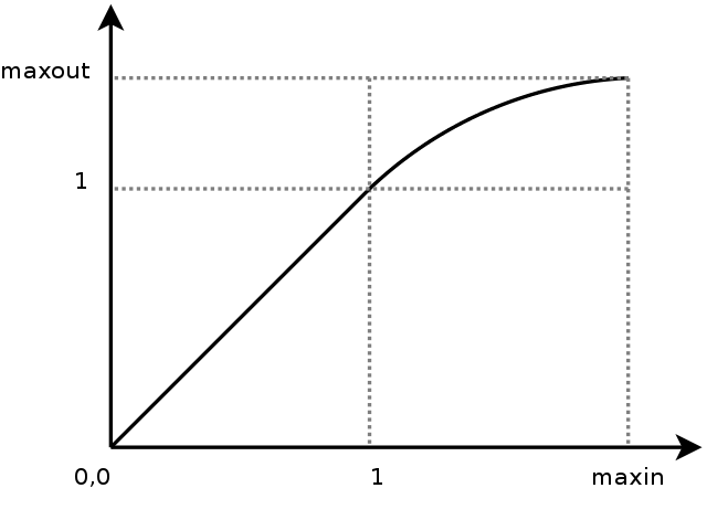
The goal is to create a compression curve that will start at a threshold of 1 with a slope of 1 (the differential is thus 1) and arrive at the maximumvalue with a slope of 0 (the differential at maxin is thus 0). The curve should be 'smooth' accross the entire compression range. Preferably in such a manner that the change from one value to the next is merely a matter of multiplying.
To approach this problem we will only deal with the segment between 1 and maxin (which maps to 1,maxout) and translate that segment to the origin. The two new boundaries are called in (i) and out (o). Their values are respectively maxin-1 and maxout-1. The segment we will create is called f, and it has intially the following requirements:


After a number of failed attempts to fit quadratic curves, cubic curves, logartihmic patches, exponential curves (e^x) and power (x^r) curves to these requirements, we determined a number of extra requirements


In words: never overshoot the maximal output value (maxout) and be strictly increasing. An extra requirement that we found was that, allthough the function must be strictly increasing, it must do so in a manner that is gradual, thus we also want that the speed by which the function slows down is strictly decreasing.

Strategy
The strategy that finally succeeded in cracking this beast was to create an appropriate differential function f' (striclty decreasing, reaching zero at the appropriate time). The integral of f' would then be the compression curve and will reach a certain maximum value at value i. That point should then coincide with the required output value o. To make it possible to reach that outputvalue we should be able to control the volume under f'. The easiest manner to achieve this, is to parameterize the bend of f'.
Also here, a number of attempts were made to use quadratic, cubic curves etcetera. Nevertheless, none were really satisfactory because we also learned that f' had to be symetric around the diagonal. This can be written as f(f(x))=x. That brought us to the following strategy.
We first create a diagonally symmetric function f' that is parameterized by a 'bend' factor. That bend factor allows us to modify the volume under f'. As soon as we then integrate f' we obtain the compression curve f and can choose the correct bend value as to reach the outputvalue o.
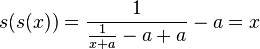
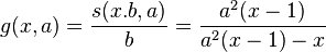
A symmetrical function
We are looking for a symmetric function s(s(x))=x . Because the function 1/x is such a function, it is worthwhile to start working from there. However, because we eventually will want to have s(0) with a sensible value (and not infinity), we also add an extra term. That term, if sufficiently large will likely help us to affect the bend of the curve.

Allthough this function is not exactly what we want it is a diagonally symmetric function
| ||||
| Two demonstrations of s(x). Note that s(s(x))=x |
The above picture shows two instantiations of this function. The left one with a=0.1. The right one with a=0.4.
Bringing s within proper bounds
The problem with s is that its value at 0 is not always 1 and that its zero crossing is somewhat arbitrary as well.
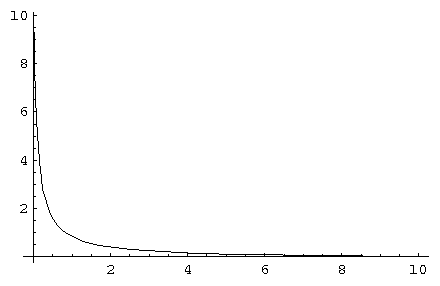
The differential we are creating (called g) must go through 1 at 0 and reach 0 at 1. Allthough the original requirement is that it should reach 0 at i, we will briefly create the function based on a target of 1 and rescale it later. Thus


To bring the value at s(0) to 1 we first divide the output of s by s(0,a), which is the value.

Secondly we also need to multiply the input of s with this value such that its value at 1 will be zero as well. That brings us to a curve g
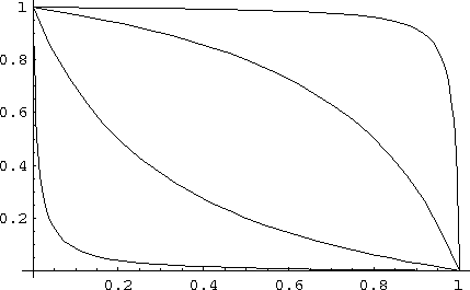 g for values 0.1, 0.5, 2 and 10
|
The parameterized differential
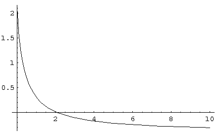
function g starts to satisfy our requirement that the slope at 0 is 1 and that we can change the volume under the curve by tuning a parameter (a). As it is currently written its zerocrossing always happens at 1. This is slightly wrong since the zerocrossing should happen at in (i). That can be achieved by scaling the inputvalue to s slightly differntly
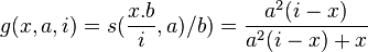
 g for values a=0.1, a=0.5, a=2 and a=10. The maximum input value was 2 for each curve.
|
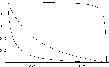
A compression segment with incorrect maximum output
The compression segment is now the integral of g. Thereby we assume that a>0 , that a!=1, that i>0, that x<i and that x>0.
 Demos of the compression segment f, with value for a=0.15, a=0.5, a=2. i=2 in all cases.
|
A compression segment with correct maximum output
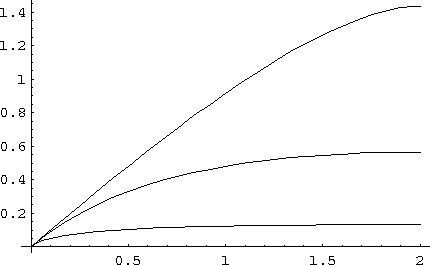
To obtain a correctly scaled compression segment, it is tempting to merely scale the output of f. That would however screw up the requirement that f'(0)=1. Consequently we are looking for the correct value of a that will lead to an output value of correct order. The maximum output is found at position i.
As can be seen, the maximum output is linearly dependent on the maximum input. That means that it suffices to find a solution for the unscaled maximum, given by
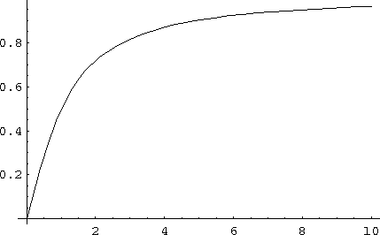 The function m(a). Horizontal it shows a. Vertically, what the maximum output value will be given that a
|
The problem now is that solving m is not straightforward, and as far as I see it, requires numeric approximation. Nevertheless, once the a-value is found for which m(a)=o/i, then that value can be inserted into f, together with i and we have the segment calculated as required.
Boundaries
- Interesting is that the limit of m is 1, we can thus never deal with sitautions where maxOutput>maxInput.
- A problem when approximating m^-1 numerically is that we encounter a division by zero around 1
- When a equals 1, f will result in a division by zero. In that case the limit of the function should be used:

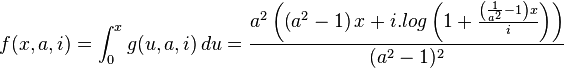
Lastly, the segment f is only part of the total compression curve given as:
Warning: rename(/home/werner/public_eq/.png,/home/werner/public_eq/php-be1893c72ccbc97fa1006849172fe179.png): No such file or directory in /home/werner/public_html/bin/images.php on line 172

| http://werner.yellowcouch.org/ werner@yellowcouch.org |  |