| Home | Papers | Reports | Projects | Code Fragments | Dissertations | Presentations | Posters | Proposals | Lectures given | Course notes |
|
|
Zathras-1: time stretching audio through matrix-multiplicationWerner Van Belle1* - werner@yellowcouch.org, werner.van.belle@gmail.com Abstract : Zathras-1 extends BpmDj with a time stretcher that does not modify the pitch of the sound. This article describes how we implemented a sinusoidal modelling by measuring the amplitude and phase envelope of peaks.
Keywords:
time stretching, audio speed change |
Table Of Contents
Overview
|
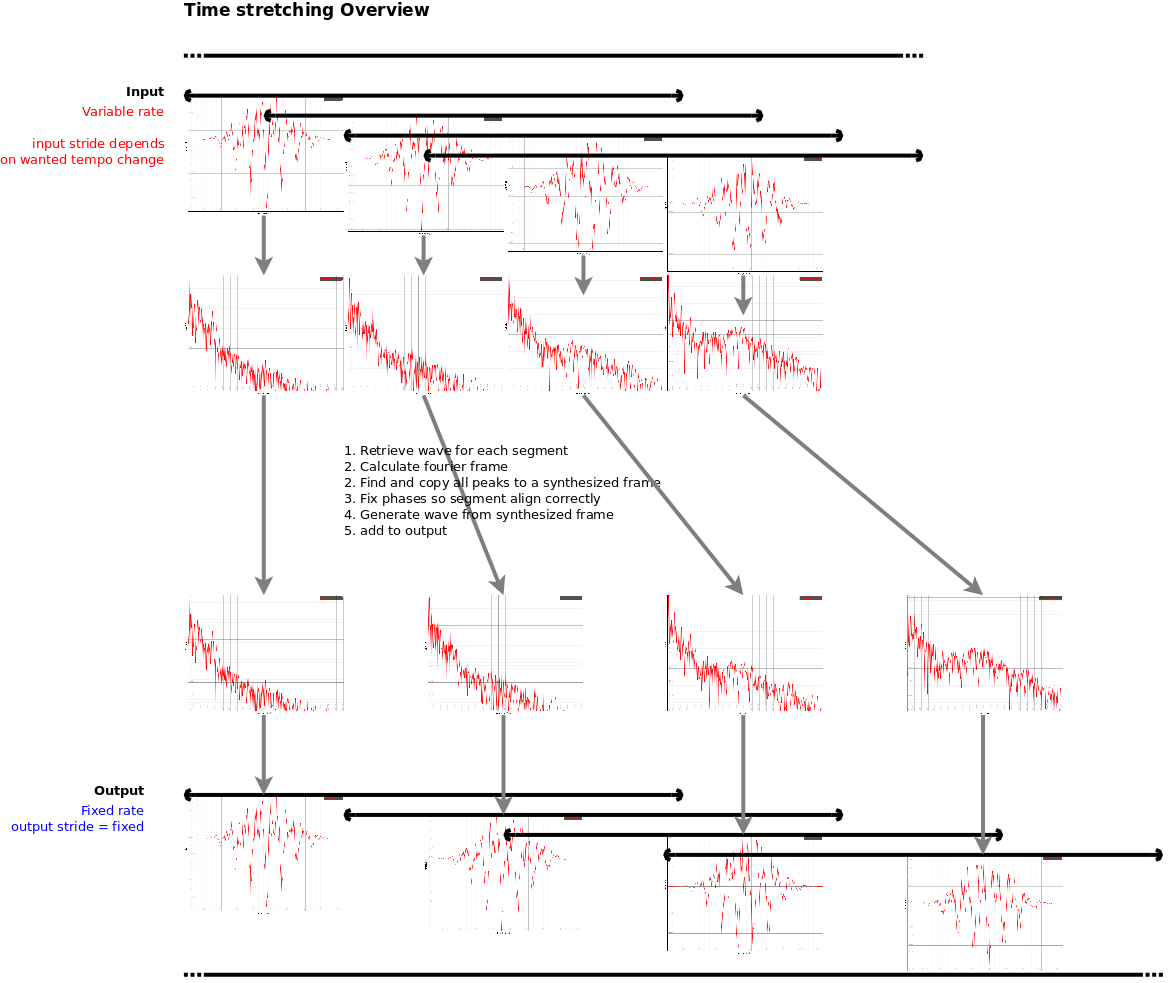
The timestretcher builds around a sliding window fourier transform. From the input signal, overlapping wave segments are retrieved, each of which is converted to its spectrum. Each frame contains multiple peaks. Each peak its envelope is analyzed, time stretched and then synthesized. Then the phases of the analyzed peak are investigated and aligned against the phases of a synthesized peak from the previously synthesized frame. Once all peaks are copied, the synthesized frame is converted to a wave and added to the output.
The output stride is a constant, while the input stride is variable. E.g: with a window size of 4096 samples and an overlap of 4, we have an output stride of 1024 samples. If the input stride is 1000 samples then the song will play at 97.65% of its original speed.
Notation
The spectrum of a discrete time domain signal  is given by Fourier's great mathematical poem:
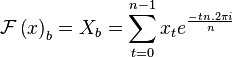
Generally, we will use a capital letter to refer to the spectrum, and a small letter to refer to the time domain representation.
With the above definitions we have the convolution theorem
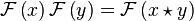
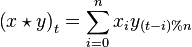
This can also be written as

The complex conjugfate of  is written as
  .
.
Reversed signals are written with an overline. E.g:  .
.
We will also use a unit sample at a specific position:  is a vector with a 1 at position
  .
.
Sinusoidal modelling
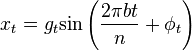
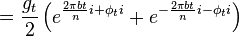
Sinusoidal modeling aims to model a signal x as a sum of sine waves
 ,
,  and
and  are the parameters of 1 sine wave. They are respectively the gain, the frequency and the phase. This model can be generalized such that not only the gain is time dependent, but also the frequency/phase combination.
Given an input signal, there will be many solutions to this model. The main challenge is to find appropriate models  , such that we can modify the time, pitch parameters in a manner that is acoustically sensible.
Gain modulation
| ||||
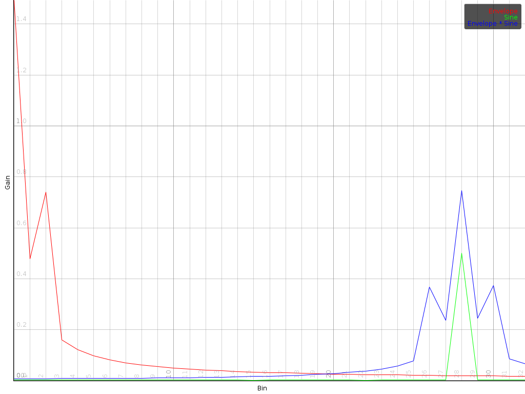
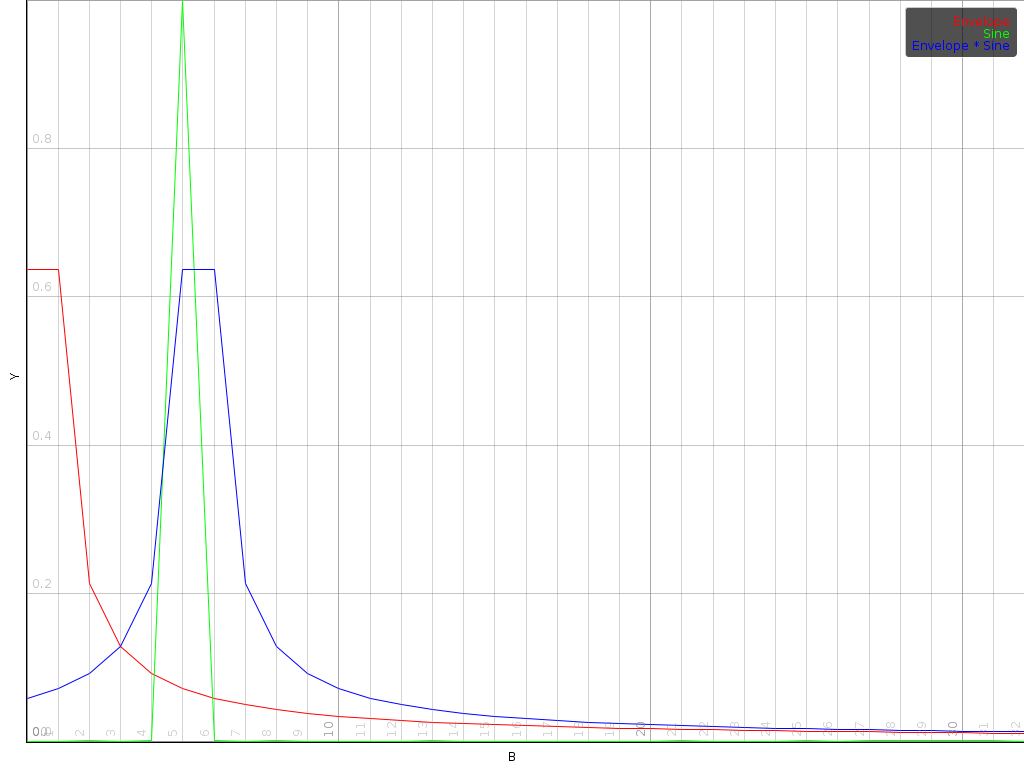
| Illustration of a sine wave (green) modulated with an envelope (the red signal). The result is shown in blue. Left the time domain version. Right, the spectrum. As can be seen, the envelope spectrum is merely shifted to the location of the sine wave in the spectrum |

To obtain the phase and gain modulation different techniques can be used. Some people don't extract those parameters and simply rely on the sequence of Fourier frames to generate appropriate gain and phases [1, 2]. Some use linear prediction [3], others map a parabola through the peak of a Fourier bin to better estimate the actual frequency [4]. In this paper we develop a novel method that determines the gain and phase envelope directly from the spectrum.
The underlying idea is that a modulation of a signal in the time domain is expressed as a convolution in the frequency domain:
In our case we assume that we have a signal ,
which is a complex oscillation at frequency bin (thus  and its spectrum is
 ). We further assume that
 has been modulated through an envelope
 , which we don't know yet.

Writing the product of and as
a convolution of their spectra and then taking the Fourier transform
of yields
| Equation modulation: |  |
Thus, if  is known, then convolving
 with will merely shift
to position (it is after all the
only non-zero bin in ). Turning this around, when
with will merely shift
to position (it is after all the
only non-zero bin in ). Turning this around, when
 and are known, we can retrieve
by shifting bins to the left.
and are known, we can retrieve
by shifting bins to the left.
Phase modulation
The modulation equation above shows how an ampitude modulation is encoded as a convolution of the envelope spectrum with the spectrum of the sine. Yet that is not all there is to it. The equation also includes a phase component. When complex is, then the phase and gain of  are
are

| ||||
To demonstrate how we can modify the frequency of our sine model,
let us assume that adds  rad
over n samples to . That is done by defining
rad
over n samples to . That is done by defining
 . The picture shows how the
central peak is blurred into neighboring channels. In a sense, we
modified the frequency of whilst preserving an
envelope gain of 1.
. The picture shows how the
central peak is blurred into neighboring channels. In a sense, we
modified the frequency of whilst preserving an
envelope gain of 1.
We could as well have started with a frequency for of 5.5 bins (instead of 5 bins) and have an envelope modulation of
1. Theoretically, in such situation our assumption to deconvolve
 by shifting it to the origin is no longer
valid, because there is no longer only 1 bin in non-zero. Yet it does not matter. We can still shift the peak to the
origin, assume its frequency was an integer multiple of
by shifting it to the origin is no longer
valid, because there is no longer only 1 bin in non-zero. Yet it does not matter. We can still shift the peak to the
origin, assume its frequency was an integer multiple of
 and then investigate the phase modulation to
determine the correct frequency.
and then investigate the phase modulation to
determine the correct frequency.
Modulation of real signals
A complex oscillation can be efficiently phase and gain modulated
in the frequency domain. When we work with real signals we should
investigate its conjugate symmetry. That is:
 and since the end result
is also real, it follows that
and since the end result
is also real, it follows that
 . Yet that means that if
 , itself must be
conjugate symmetric as well. That further means that must be real. In other words it would be impossible to introduce a
phase modification if we were to merely convolve two conjugate
symmetric peaks.
, itself must be
conjugate symmetric as well. That further means that must be real. In other words it would be impossible to introduce a
phase modification if we were to merely convolve two conjugate
symmetric peaks.
Luckily, it is possible if we only look at half of the
spectrum. Assume that is a real valued signal that
consists of a gain ( ) and phase modulation
(
) and phase modulation
( ) of a sine wave of frequency .
If we now define  then
then
The Fourier transform of this is

While the first peak is modulated with the forward envelope. The second peak has to be modulated with its reverse conjugate.
Extracting peaks
Envelope Sampling Rate
That the envelope of a signal is a localized phenomenon in the spectrum, makes it possible to extract it, together with its sine wave, as a single peak from the spectrum. By shifting the peak to the origin, we get rid of the sine wave and solely model the envelope.
Assume, we find a peak at position in the
spectrum of . If we extract a window from
 to
to  , we
get
, we
get
models the envelope at a sample rate of
 . If we use only 1 bin, at a sample rate
of
. If we use only 1 bin, at a sample rate
of  and a window size
  ,
then we sample the envelope at 10 Hz. Using 4 bins allows us to sample
the envelope at 40 Hz and so on. In practice we will not always choose
a fixed modulation sample rate. Instead, the width of the extracted
modulation spectrum will depend on the position of local peaks.
,
then we sample the envelope at 10 Hz. Using 4 bins allows us to sample
the envelope at 40 Hz and so on. In practice we will not always choose
a fixed modulation sample rate. Instead, the width of the extracted
modulation spectrum will depend on the position of local peaks.
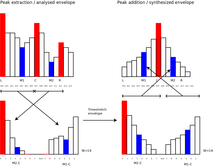
Envelope Extraction
|
5 positions in the originating frame are defined.
 is the bin of the left peak (a local maximum).
 is the position of the minimum between left and middle
peak.
is the position of the minimum between left and middle
peak.
 is the position of the middle peak/the peak we
are extracting.
is the position of the middle peak/the peak we
are extracting.
 is the position of the minimum
between the middle peak and the next peak and
is the position of the minimum
between the middle peak and the next peak and
 is the
position of the next peak.
is the
position of the next peak.
When extracting a peak, we place it in a Fourier frame of
appropriate size. Source bins and are the previous and next peak. They will receive a weight of 0, and
thus don't need to be transferred. The right side of the peak, from
to will be placed in the positive
frequencies of the target spectrum. The left side of the peak, from
to , will be placed in the negative
frequencies of the target spectrum.
The middle bin of the target spectrum (with radian frequency
) cannot be used because it is both a positive and
negative frequency at the same time. When synthesizing a new peak,
this bin would be a problem because we would not be able to figure out
whether its value belongs to the left or right side. From all this it
follows that we need at least  positive
frequencies and at least
positive
frequencies and at least  negative
frequencies. The smallest higher power of two larger than twice the
maximum of these two values is the size of the envelope spectrum we
need.
negative
frequencies. The smallest higher power of two larger than twice the
maximum of these two values is the size of the envelope spectrum we
need.
Weights
In a frame many peaks are present. The values between two peaks should be correctly assigned to each of them.
One method could be a linear weighing. That would mean that the middle between the two peaks is assigned 50% to the left peak and 50% to the right peak. That is however a slightly inappropriate approach because sines tend to behave as decaying exponentials when they do not perfectly align to a bin.
A better assignment is determined by obtaining the position of the minimum between peaks. The interpolation of the values between one peak and the other is then given as an exponential curve, which goes through the minimum position with a value of 0.5.
For the left flank we define  and
and  . For the right flank we define
  and
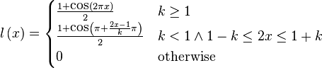
and  . The following function, defines how to weigh the contribution of each value, given its location .
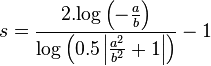
This curve is loosely based on our article 'Fast exponential envelopes' [5].
| ||||
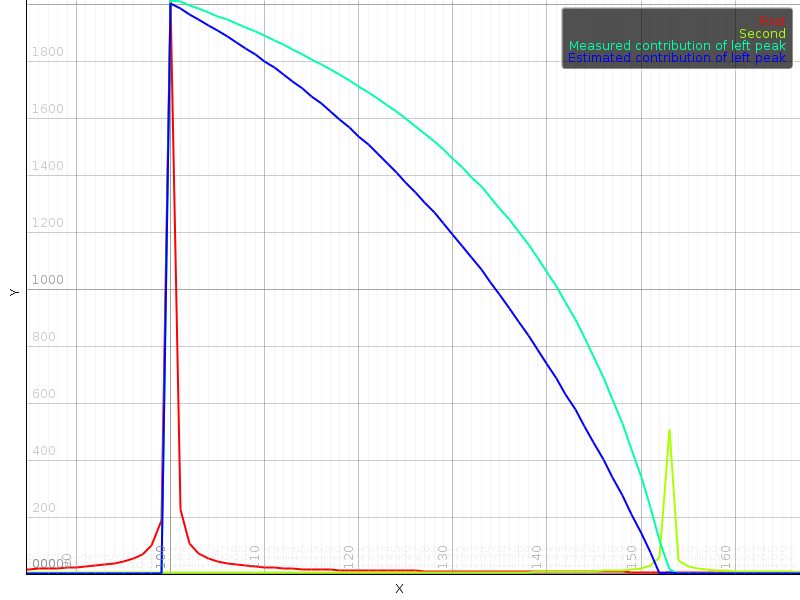
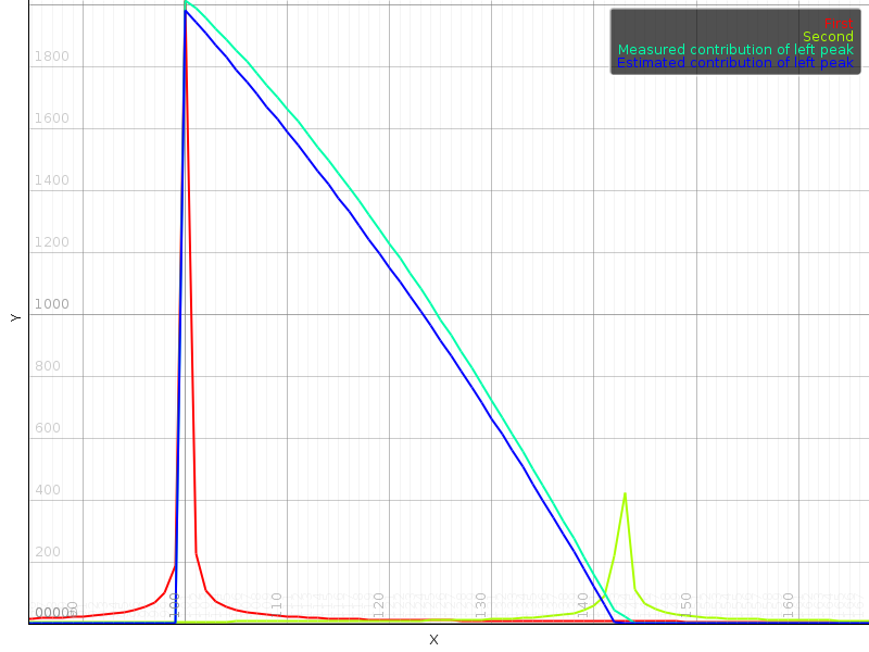
That this is a good model can be seen by generating sine waves of different frequencies and then plotting the contribution of each sine to the value of a particular bin. In parallel, we can plot our estimate  . Such an experiment shows that the main inaccuracy of our model appears when the actual minimum position falls between bins, close to either peak. In that case the observed local minimum is not necessarily the exact location of the minimum.
With all this in mind we can now write down the extraction of a single peak. Values are extracted starting at the previous peak (excluding the peak itself) up to the next peak (again excluding the peak itself).
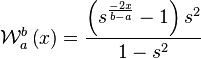
Time stretching/shrinking the envelope
Once we have the spectrum of the envelope (), we can compute the backward Fourier transform to obtain a time domain representation (). Then we can create a new envelope  , which is a time stretched version of . Because shrinking time might increase the frequency content of , it follows that and are not necessarily of the same size. The size of will be denoted
  . The size of denoted
  . and are nonetheless powers of two and might be larger than strictly necessary.
Position Mapping
Assume the time stretch ratio is given by  . When
  , the song plays slower,
  the song plays faster. The time stretch ratio can be obtained by comparing the input stride against the output stride.
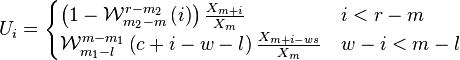
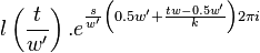
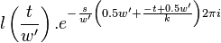
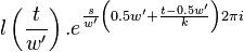
The position mapping between the original envelope and the new envelope is given by calculating the distance to the middle position and then rescaling it. The following equation specifies the source position (in ), when a target position  (in ) is known.
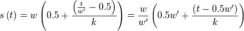
In the above, the factor retrieves the data from the correct position in the source envelope.  is a window to smoothen out the edges.
Windowing
“I have to find the edge of the envelope and put my stamp on it.” ― Terry Pratchett, Raising Steam
|
The first reason to apply a window is that might
not always have a multiple of  radians in total;
nor do we have any guarantee that the amplitude at the end of the
frame will match the amplitude at the beginning of the frame. In
other words: in all likelihood
radians in total;
nor do we have any guarantee that the amplitude at the end of the
frame will match the amplitude at the beginning of the frame. In
other words: in all likelihood  will be
discontinuous. That in turn might lead to strong oscilations of the
gains/phases throughout the entire envelope. This problem is
effectively mediated by means of a hann window.
will be
discontinuous. That in turn might lead to strong oscilations of the
gains/phases throughout the entire envelope. This problem is
effectively mediated by means of a hann window.
A second reason is that we don't always have the information we
need. When shrinking time we will have positions in
that map from source positions outside the
analysed frame. Because we cannot say much about such locations, it
is useful to set them to zero, as picture above.
The intermediate window is thus defined as
With this definition we have that 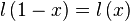 .
.
Resampling
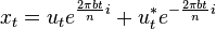
The last problem involves the resampling of . Although the target position will be an integer, the source position might not be. That means we that we must interpolate . The Fourier coefficients make this easy:
In equation [eq:resampling-integral], we directly wrote the Fourier integral as a summation of the positive and negative frequencies. From a computational point of view this is useful because we only need to calculate/retrieve one coefficient and compute two terms with it. A second reason we explicitly split positive and negative frequencies is because resampling works only correctly when falls within  to . Multiplying an aliased frequency with a non integer number will result in the wrong frequency being generated. E.g:
 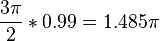 . Whilst
  . Yet
. Yet  is not an alias of
  .
.
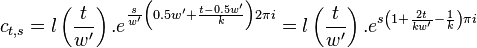
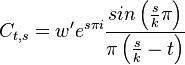
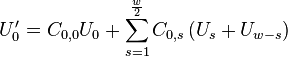
Coefficients
We can now determine the value of 
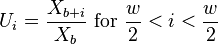
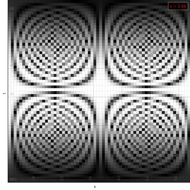
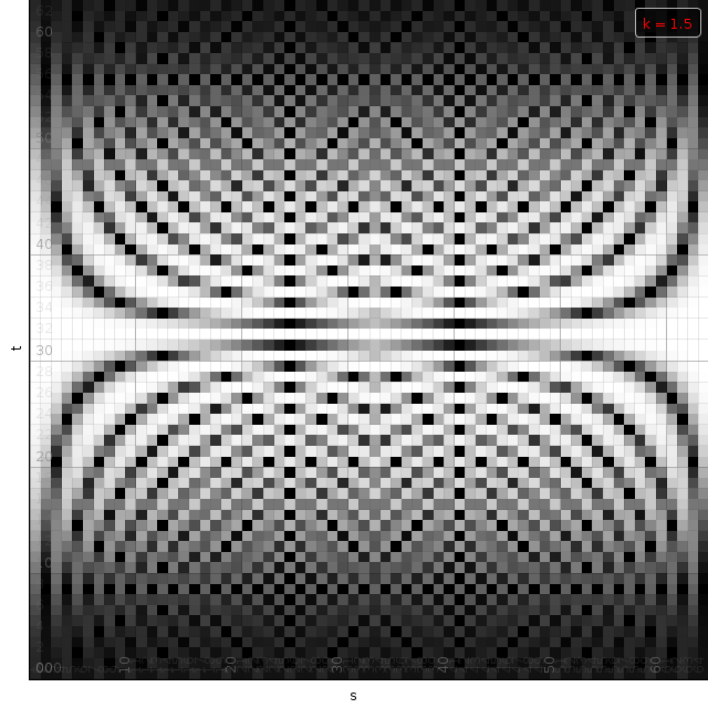
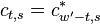
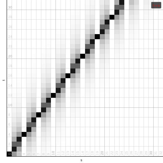
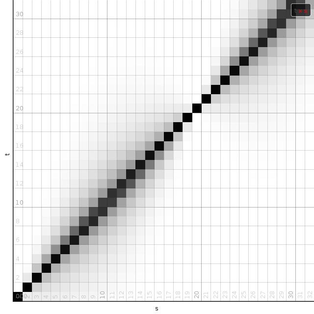
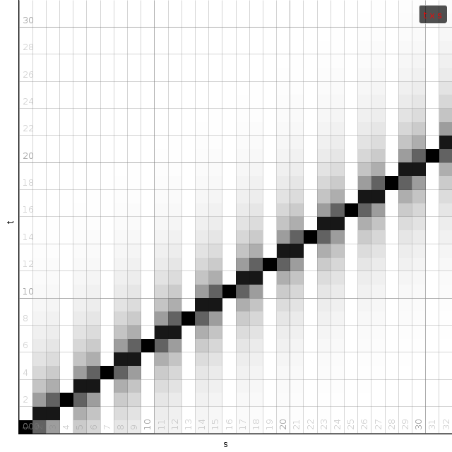
We can set up a matrix  that will allow us to compute from as a straightforward matrix multiplication. For a fixed and we define the following coefficient matrix.
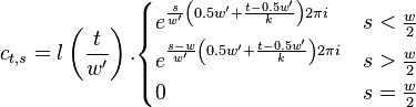
With this definition is defined as

| ||||||
| Demos of the c matrix for time stretch factors k=0.75, 0.99 and 1.5. White reflect values with a large norm. Dark are values with a small norm. The intermediate window I can be perceived as dark bands at the top and bottom of each image. |
Symmetry relations
There exist 2 symmetry relations in that can help speed up resampling of into the time domain of .
The first symmetry property is that
For  this is trivial since
  . For
. For  we have
 |  |  |
 | |  |
 | |  |
 | |  |
For  we have
 | |  |
 | |  |
 | |  |
 | |  |
| |  |
The second symmetry relation is
| |  |
 | |  |
 | |  |
In summary, given a fixed time stretch ratio , an input window size of and output window of , we only need to obtain ,  and
and  to calculate and
  .
.
Stitching
 fabrics doesn't make exquisite dresses, it is the stitches.
|
With the ability to extract a sinusoidal components from a frame, and synthesize them into a timestretched signal, we should now look at piecing together consecutive frames. Or in our particular case how to determine a previous peak to which to attach, and how to bring the phases of the new peak in alignment with the old one.
To determine a previous peak we merely look at the previous frame and find the nearest peak, irrespective of its phase or volume. With our time stretcher there is no need to set out a path or try to detect whether traces are dying or coming to live [2]
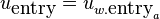
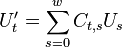
To align the synthesized waves, we must know the entry and exit phases of the analysis stage as well as those of the synthesis stage. To determine these, we will deal with 4 positions, each dependent on the relevant stride.


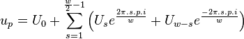
These positions are relative to the frame (they range from 0 to 1),
so they must be multiplied with  to obtain a correct
sample position. They have been created such that when an input or
output stride is applied, the exit position of the previous frame
overlaps with the entry position of the new frame. The subscript
denotes whether we deal with the analysis or synthesized frames.
to obtain a correct
sample position. They have been created such that when an input or
output stride is applied, the exit position of the previous frame
overlaps with the entry position of the new frame. The subscript
denotes whether we deal with the analysis or synthesized frames.
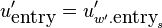
To lighten the notation of the upcoming discussion, we will
automatically use the appropriate analysis or synthesis positions:
 and
and
The phases of the translated peak are not the phases we would
measure in itself. When the peak is repositioned to
position , then the fully correct phase of the output
requires us to add  , multiplied with the
entry/exit position, to the angle of . Therefore, the
entry and exit phases of the analyzed peak and the synthesized peaks
are:
, multiplied with the
entry/exit position, to the angle of . Therefore, the
entry and exit phases of the analyzed peak and the synthesized peaks
are:


Because we will now discuss how we make sure that the various waves align correctly, we need to discuss the entry and exit positions of the analysis and synthesis spectra of the previous and current frame. Current peak values are annotated with a superscript \'cur\'. Previous peak values are annotated with a superscript \'prev\'.
The start phase of the synthesized sine ( ) must be in alignment with the exit
phase (
) must be in alignment with the exit
phase ( ) of the
previously synthesized wave. Or to be more correct, it should have the
same error as the entry and exit phases had during the analysis stage,
which is given by
) of the
previously synthesized wave. Or to be more correct, it should have the
same error as the entry and exit phases had during the analysis stage,
which is given by  .
.
The current entry phase of the synthesized sine is
 yet it should be
 . Thus we must phase shift the
synthesized wave by
. Thus we must phase shift the
synthesized wave by

To expand the full phases, we need to know the positions of the
previous peak ( ) and that of the
position of the current peak (
) and that of the
position of the current peak ( )
)

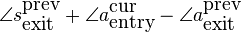
Reorganizing the various terms and using the fact that exit=1-entry, gives us the required phase modification of the synthesized peak:

In words this reads as: the required phase modification is the sum of 1) the entry phase differences between the synthesized and analyzed envelopes of the current frame and 2) the exit phase differences between the synthesized and analyzed envelopes of the previous frame, and 3) the peaklocation difference multiplied with an appropriate phase trend.
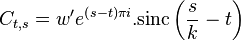
Resampling the envelope as a matrix multiplication
The calculation of a time domain representation of
from the spectrum of is
straightforward, yet it requires a backward Fourier transform from
to  , before adding it to the
output frame. It is possible to omit the conversions
, before adding it to the
output frame. It is possible to omit the conversions
 and
and  completely.
This is done as follows. has been previously
defined as

has rows and
columns. has rows.
Taking the Fourier transform of both sides gives
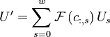
Thus by computing the Fourier transform of each column in the
matrix , we can directly compute
. Interesting thereby is that since each column in
is conjugate symmetric, the Fourier transformed
matrix will consist entirely of real numbers.
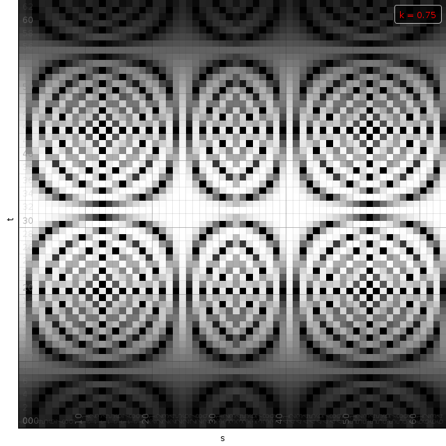
Fourier transform of c
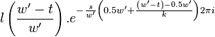
| ||||||
| Some examples of the matrix C, given a window size of 64 bins and various tempo modifications. Dark are large values. White are small values. Only a quarter of the full matrix is shown. All other quarters are determined through various symmetry relations. |
To compute the Fourier transform of we will
only determine the transform for values of
 . How the other half can be ignored will
be explained later.
. How the other half can be ignored will
be explained later.
Were we to include the intermediate hann window in the integral directly, then might not be able to solve it
easily. Yet, since is a multiplication of two
functions, their Fourier integrals will be a convolution. Therefore,
we currently omit the hann window, and will later smear the bins
appropriately.

Which further reduces to
Subtracting  from the value we pass into the
sine does not change the outcome, but might swap the sign, depending
on the oddity of . Similarly, the oddity of
also determines the sign of the outcome. Overall we
get the following:
from the value we pass into the
sine does not change the outcome, but might swap the sign, depending
on the oddity of . Similarly, the oddity of
also determines the sign of the outcome. Overall we
get the following:
Application of window requires us to calculate
the convolution of the neighboring bins. Luckily the convolution
window is very small. With coefficients such as -0.25,0.5 and -0.25 we
can easily smoothen  with
with
 .
.
Because  is a sparse matrix it makes parameter
changes to easy to deal with. Only a selected few
old coefficients must be removed and regenerated at a new
position.
is a sparse matrix it makes parameter
changes to easy to deal with. Only a selected few
old coefficients must be removed and regenerated at a new
position.
Symmetry relations
From the fact that , it
follow that  is real. From the symmetry
relation
is real. From the symmetry
relation  , follows that
 because
 . These
two symmetry relations are useful to reduce the size of the matrix and
speed up computation:
. These
two symmetry relations are useful to reduce the size of the matrix and
speed up computation:


Thus by obtaining coefficients and
 , and combining them with the input values
and , we compute terms
for
, and combining them with the input values
and , we compute terms
for  and
and  . When
 we can reduce this even further to
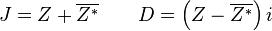
Stereo tracks
The described method recreates sound with high fidelity, yet it does not honor the phase content of a track. Time stretching a stereo track by processing each individual channel makes the sound appear phased and out of the room. Reverbs will sound wrong and the overall ambiance will be affected. To solve that, to a certain extent, it is useful to merge stereo tracks and then time stretch the merged and difference signal individually. Once time stretched, we can again calculate the left and right channel.
The joined and difference channel are defined as:


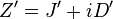
To obtain the Fourier transform of these two at the same time we
can calculate the Fourier transform of
 . (This trick is taken from [6]).
When a new  and
and  have been
created, we need to restore a left and right signal. This again can be
done with 1 Fourier transform
have been
created, we need to restore a left and right signal. This again can be
done with 1 Fourier transform
The inverse transform of of  has a real part
that will be
has a real part
that will be  and an imaginary part that is


This entire process of joining and mangling the input channels and
output channels introduces a gain of 4, which should be compensated
for with the normalisation gain into .
Normalisation gain
Aside from the stereo convertion and the 2-for-the-price-of-one FFT tricks, other operations also affect the gain. In particular the various windows used by the time stretcher:
The first window applied is the analysis window. It is necessary to use a hamming window here because its first side lobe is removed. Compared to other windows, this one makes detecting peaks easier and makes interpolation between peaks more accurate. The necessary gain compensation for the analysis window depends on the time stretch ratio.
The second window we use is a modified hann window
. It is applied to the synthesized peaks such that
the Fourier representation can deal with the discontinuity at the edge
of the frame.
The last window is the synthesis window. We choose a welch window, mainly to get rid of phase cancellation artifacts. Whenever we select a wrong peak or have an insufficiently large peak window, we find that we retain some waves that would ordinarily have been canceled out. These problems are mostly apparent at the edges of the synthesized window. A welch window offers a great solution to this whilst retaining as much overlap as possible between frames.
Another place where we omitted gains are the forward and backward
Fourier transforms. A forward transform followed by a backward
transform introduces a gain that matches the windowsize. This becomes
especially confusing when matrix converts a smaller
envelope to a larger one.
Latency
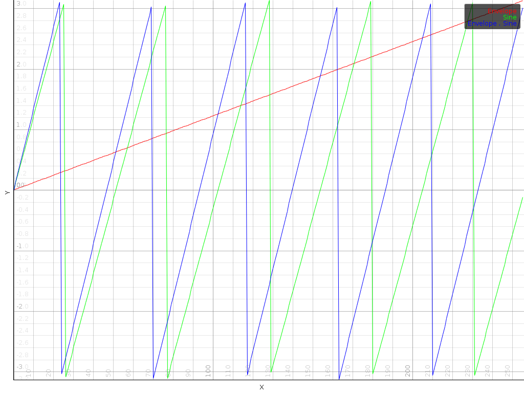
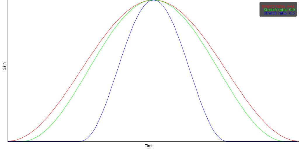
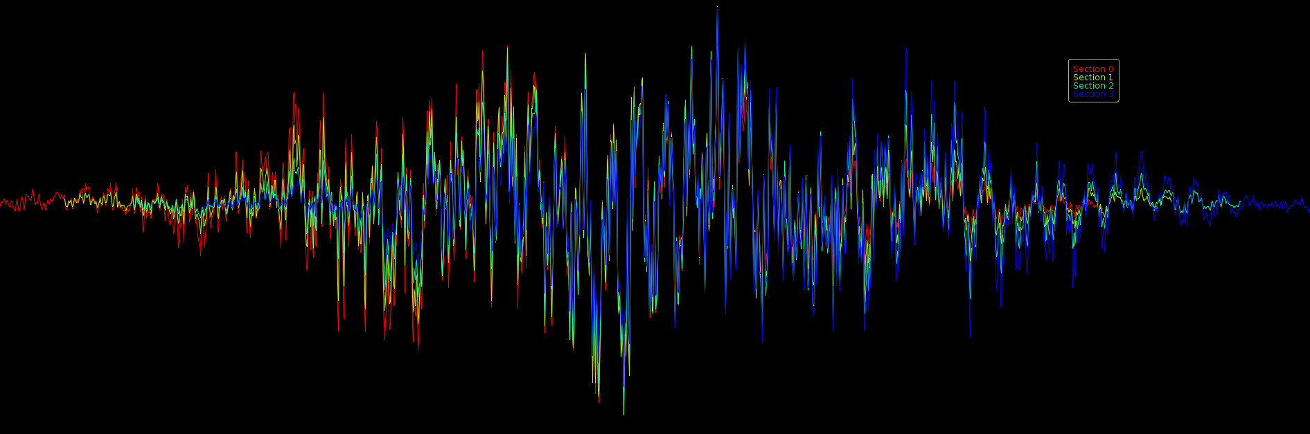
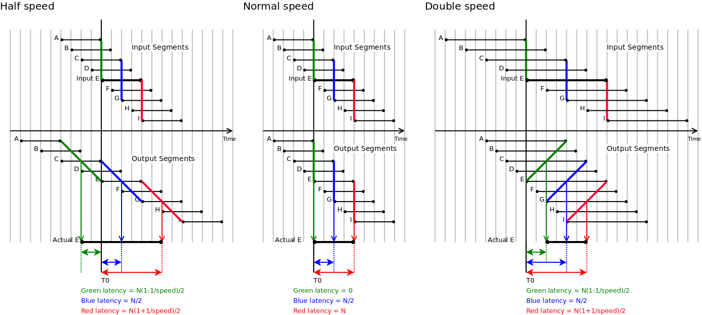
The latency calculations can be fairly tedious depending on where we anker ourselves. That is, when we input data into the timestretcher, do we measure the latency until the first sample of our input comes out, the middle or the last sample ? Contrary to most latency calculations, if we do not take the middle sample as a reference point, we will have a latency which is affected by the playbackspeed.
|
To get a grasp on the latency, we drew a number of scenarios: halve speed, double speed and normal speed. For each scenario we placed ourselve at time 0. At T0 we put frame E into the timestretcher and see how it comes out, and more importantly, how it interacts with previous and future frames provided to the timestretcher. Here it must be noted that allthough the graphics might suggest that the input frame stride is fixed, in reality it is the output stride that is fixed. Also the length of all segments is fixed, independent from the playbackspeed.
For a 0.5 playback speed, we see that the starts of the output segments, compared to the starts of the input segments, are stretched out in time. While each input sample is offered to ~5 frames, each output sample only comes from ~3 frames. The graphic shows how the beginning of segment E (drawn in green) is placed at 5 output positions, with a center in the middle of C. The middle of segment E, drawn in blue, appears in the output frames also at different positions. However, in this case, its center is still centered at E. Lastly, the end of segment E maps to the middle of G in the output. Practically, speaking, segment E will be stretched out in time, starting at N*(1-1/speed)/2, up to N*(1+1/speed)/2 (with N referring to the framesize, typically 4096 samples). These bounds define the latencies of the timestretcher.
Similar scenarios are plotted at normal and double speed.
In this article we presented the Zathras-1 time stretcher. The time stretcher detects and transfers all peaks from the source to the target frame. For each peak the envelope is extracted and recreated after time stretching. The phases of consecutive peaks are aligned with the same error they had in the input signal.
The presented algorithm works well with a window size of 4096 samples and an overlap of 4. It can be used to time stretch ~14.6 stereo tracks simultaneously on a 1.4GHz computer. That means that per frame we spend 1.59 milliseconds. On average we have about 630 sine waves per frame, which leaves us with a computational time of about 2.5 microseconds per peak. Results of the time stretcher can be heard here [7].
Potential improvements include a proper rescaling of the phase modulation. Currently we stretch the phase modulation, which introduces a small error. Secondly, preserving the phase-error as it appears in the source frame might be improved by tuning the error in function of the time stretch ratio. Another improvement would be to have some estimate on the probability that a local maximum is indeed a local maximum and if not switch to another time stretching method.
Bibliography
| 1. | Phase Vocoder Flanagan J.L. and Golden, R. M. Bell System Technical Journal 45: 1493–1509; 1966 |
| 2. | Speech Analysis/Synthesis Based on a Sinusoidal Representation R. McAulay and Th. Quatieri IEEE Transactions on Acoustics, Speech, and Signal Processing; August 1986 |
| 3. | Enhanced Partial Tracking using Linear Prediction M. Lagrange, S. Marchand, M. Raspaud, J.B. Rault Proc. of the 6th Int. Conference on Digital Audio Effects (DAFx-03), September 2003 |
| 4. | PARSHL: An Analysis/Synthesis Program for Non-Harmonic Sounds Based on a Sinusoidal Representation J. Smith III, X. Serra Center for Computer Research in Music and Acoustics (CCRMA). Department of Music, Stanford University; 1987 https://ccrma.stanford.edu/~jos/sasp/Quadratic_Interpolation_Spectral_Peaks.html |
| 5. | Fast Exponential Envelopes Werner Van Belle Audio Processing; YellowCouch; April 2012 http://werner.yellowcouch.org/Papers/fastenv12/index.html |
| 6. | FFT of pure real sequencey. |
| 7. | Zathras-1 Werner Van Belle Yellowcouch Signal Processing http://werner.yellowcouch.org/log/zathras/ |
| http://werner.yellowcouch.org/ werner@yellowcouch.org |  |