| Home | Papers | Reports | Projects | Code Fragments | Dissertations | Presentations | Posters | Proposals | Lectures given | Course notes |
|
|
16. Calculating Up-/Down- Regulations using qPCR /RTPCRWerner Van Belle1 - werner@yellowcouch.org, werner.van.belle@gmail.com Abstract : In this article explain the finer points of the delta-delta-CT method to calculate up-/down- regulations. The following text is a writeup of a course I gave at a local highschool.
Reference:
Werner Van Belle; Calculating Up-/Down- Regulations using qPCR /RTPCR; Bioinformatics; YellowCouch; August 2010 |
Table Of Contents
Quantitative PCR / realtime PCR
To explain the analysis process of a quantitative PCR (qPCR) we will first look into a mathematical simulation of a PCR. How would a concentration curve look like if we assumed a specific copying process. Later on, we focus on a standard up/down regulation analysis that includes the use of a houshold gene and dilution series.
Simulating a PCR
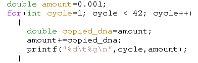
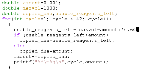
To simulate a quantitative PCR, we start off with a specific volume of DNA material: amount. With each cycle we will 'more or less' double the amount of DNA. This is the copied_dna. After a number of cycles this exponential process explodes. (click on the images to see the full sized version)
| ||||
| Simulation without any restriction. The X-axis contains the cycle count, the Y-axis plots the amount of DNA |
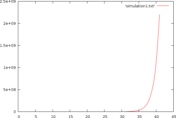
Of course the well volume is finite, which means that, as soon as there are no longer sufficent reagentia left, we should limit the DNA that is copied. Below we restrict the the amount of newly produced DNA by the maximum of the available DNA and the available reagents.
| ||||
| Simulation with hard volume limit. X-axis: cycle-count; Y-axis: amount of DNA |
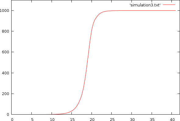
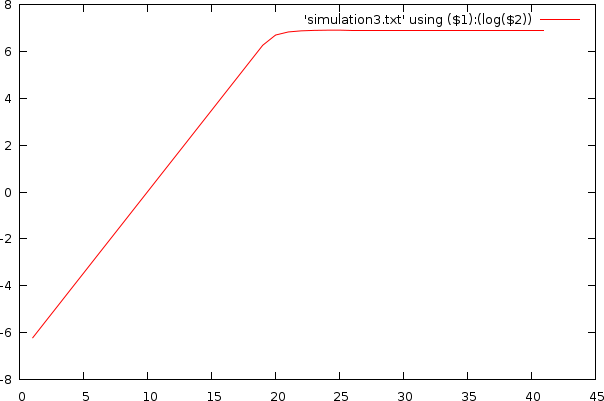
The above plot has a fairly hard limit because we assumed that anything that was not DNA was reagentia used to create new DNA. That is of course not true. In general, the usable reagents are only part of the remaining volume, which leads to the very nicely simulated expected output from a quantitative PCR, as pictured below.
| ||||
| Simulation with volume and reagentia limit. X-axis: cycle-count; Y-axis: amount of DNA |
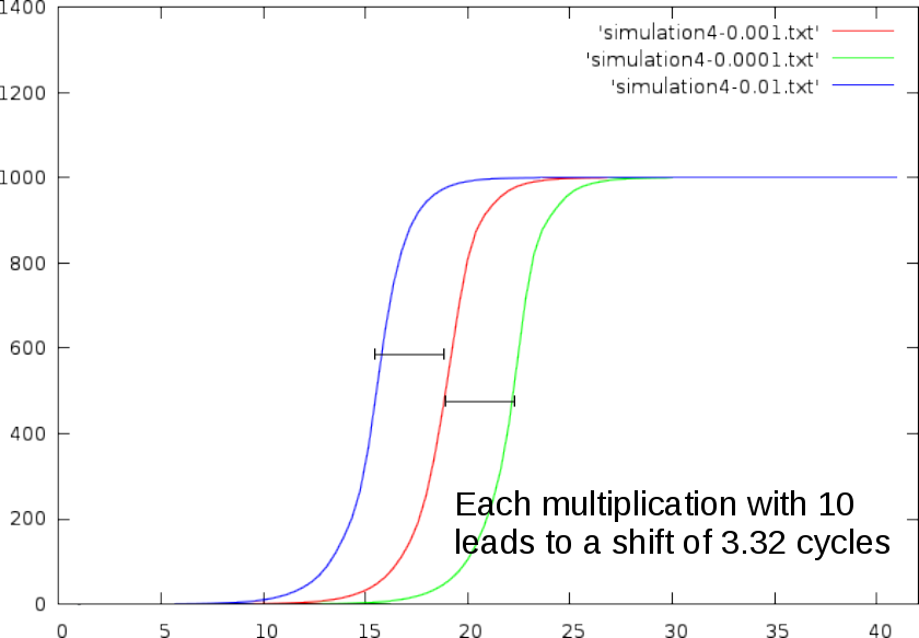
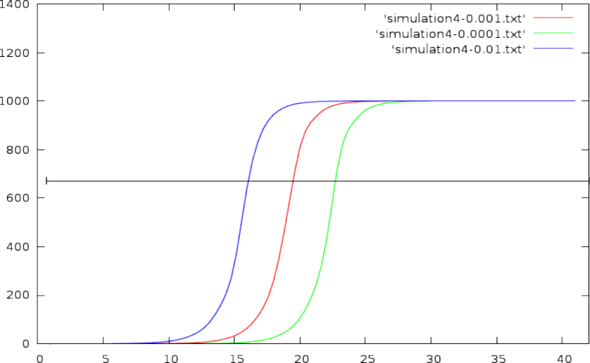
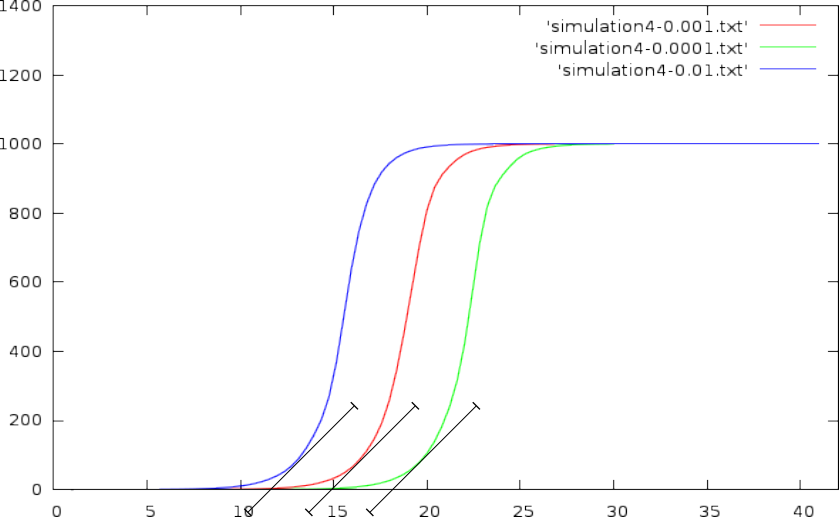
How does the initial amount affect the curve ?
The trick in quantitative PCR is that the initial concentration affects the time it takes to reach a specific target volume. This we can reverse, and thus, based on the time it takes to reach a specific amount of DNA, we can calculate the initial concentration.
A multiplication of to the initial concentration will shift the qPCR curve to the left (we need less cycles to reach the same absolute amount), or right (we need more cycles to reach the same amount).
|
In practice,
- multiplying the initial concentration with 2, shifts the curve 1 cycle to the left.
- dividing the initial concentration with 2, shifts the curve 1 cycles to the right.
- multiplying the initial concentration with 10, shifts the curve ~3.32 cycles to the left.
- dividing the initial concentration with 10, shifts the curve ~3.32 cycles to the right.
The reason we observe a curve shift (as opposed to a curve scaling) when the initial concentration is multiplied, lies in the exponential nature of the PCR process. Mathematically, we can express the exponential growth as an 'amount of DNA at cycle c' (annotated a_{c}). This amount depends on the amount of the previous cycle a_{c-1}, which in turn depends on the amount of its previous cycle a_{c-2}, etc. This dependency chain goes whole the way back to cycle 0, where a_0 equals the initial concentration. This can be written as
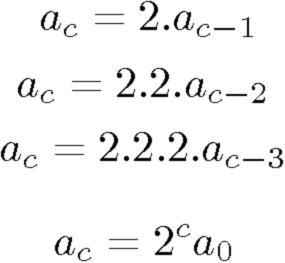
This chain of multiplications results in an amount of DNA at cycle c which is 2^cycle multiplied with the initial amount.
If we now assume an initial concentration of a0 and a target amount (T), how many cycles (c) will it take to reach that amount ?
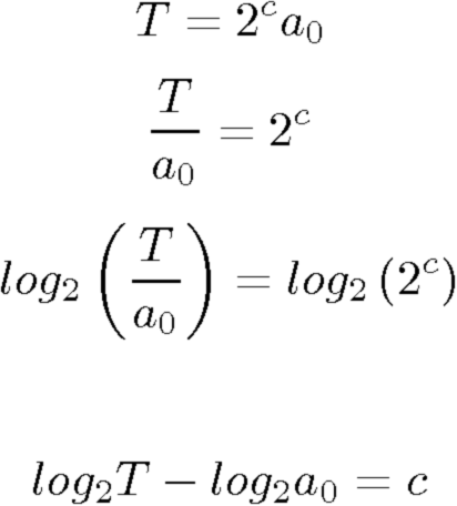
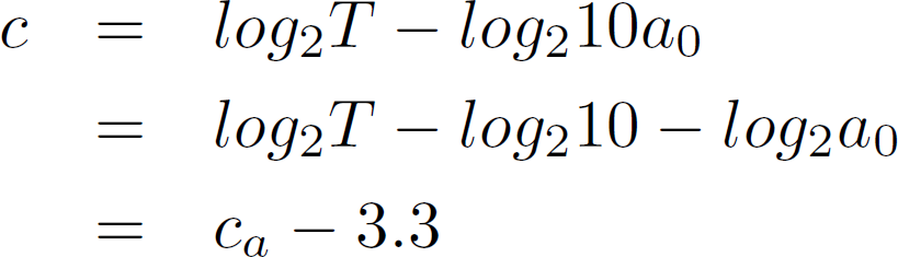
To understand the effect a concentration increase of a factor 10 has, we can simply write 10a_0 and see what it does to the cycle count.
Obtaining CT or CP Values
Using a quantitative PCR we can measure the number of cycles it takes to reach a certain threshold value. This cycle count is often called a CT value, or sometimes also a CP value. The finer nomenclature doesn't matter here. What is important is that the cycle count can be calculated back to the initial amount of DNA, and thus to the concentration that was present in the well.
There are of course two problems with this approach
- There is no such thing as 'half a cycle'. The cycle is done or it is not. The best solution to deal with this is to perform a curve fitting and estimate the accurate position of the CT value. This can be easily done by first converting the concentration to a log value and then fit a straight line to this curve.
- The exponential growth tapers off after a certain number of cycles (capped due to the volume and reagentia limit).
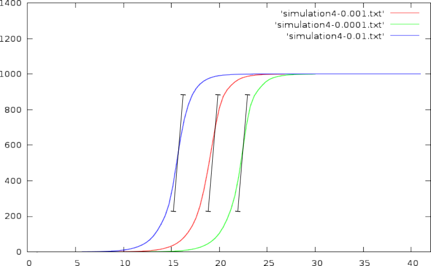
- This can be solved by choosing an absolute DNA volume to reach (a horizontal line through the graph, and pick out the CT values where this horizontal line crosses with the volume curve)
- or one could rely on a required slope.
- or one could place the CT value of a curve at its maximum slope
In this discussion it matters not how to obtain the CT value, and from my point of view too much attention is paid to this particular aspect of qPCR.
Accuracy of the CT values
Just out of cheer curiosity I tested how a small error in the CT value would affect the calculated concentration.
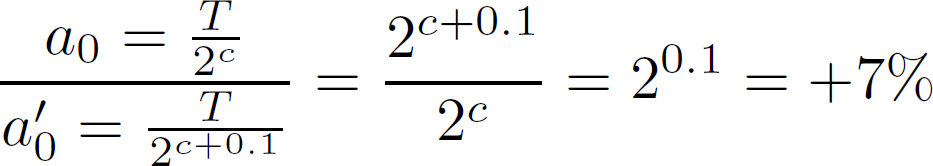
Well, staggeringly, a 0.1 change in cycle count (CT value) affects the initial concentration with 7% !
Copyrate efficiency
Another factor quite relevant to the qPCR debacle is the efficiency of the copy process itself. There are two somewhat confusing terms around:
- copyrate - refers to the multiplication factor from one cycle to the next. E.g: a factor of 2 would mean that all of the input DNA is copied. In other words: a perfect efficiency.
- [copyrate] efficiency - refers to how much of the input material is copied. E.g: an efficiency of 100% would be the same as a copyrate of 2.
In general, copyrate efficiencies of 100% are seldom achieved. Efficiencies of 90% are somewhat more realistic; and of course, we would like to understand what effect this has on a) the CT values and b) the calculated concentrations.
Based on a simulation, in which we assumed a per-cycle copy-efficiency between 95% and 100%, we found the following outcome:
With an initial concentration/amount of 0.001- At perfect efficiency we would need 18.907 cycles to reach a specific threshold.
- At a copy efficiency between 95% and 100% (randomly chosen for each cycle), we need around 19.2524 to reach the same threshold.
- The difference between these two CT values is 0.3454; which if we assumed that the efficiency was 100%, would result in a 21% underestimation of the actual concentration.
- At perfect efficiency, we need 25.49 to reach a specific threshold
- At a copy efficiency between 95% and 100%, we need around 26.0581.
- The difference being 0.5681 cycle, leads to a 33% underestimation of the actual concentration.
These errors are staggering and it should be clear by now that the mantra 'qPCR is so accurate due to its amplification process', is sheer nonsense. The amplification process will also copy errors for one, and secondly, if the amplification process has not a sufficiently stable and/or known efficiency, then any subsequent calculation will be seriously misguided (not to say wrong).
Normalization of CT Values based on dillution series
To deal with the problem of such unknown efficiencies we can fall back to our observation that the CT distance between two curves of different concentrations is around 3.3, if one concentration was 10 times smaller (or larger) than the other.
The expected distance (x) between two curves, given a concentration ratio of 10, and a copyrate of (r) would be
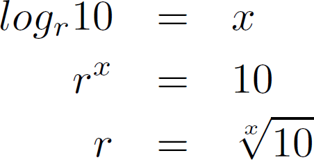
This leads to the following observed copy rates, given a certain curve-distance
Depending on the used dilution series, the above equation might need a different value for 10.
Normalizing concentrations
Based on the measurement within one curve, it is possible to observe how much material was copied from cycle to cycle and use that to estimate the efficiency of the process for that particular curve. Based on that again, we can directly calculate the initial concentration. That is however not how it is often done because such change calculations at the lower cycles is very error prone, due to a limited machine accuracy. Normally, people tend to continue working with the CT-values.
Normalizing CT values
If we want to use the delta-delta-CT method later on we must be able to normalize the CT values as if the copy process was 100% accurate. If we for instance measured a CT value of 10, at an efficiency of 95% then, expressing this at an efficiency of 100% would result in a CT value of around 9.63 cycles.
To get a grasp on this mathematically, it suffices to assume that we reach a specific volume V after x cycles, given an initial amount of i and a copyrate of r.
To reach this volume if the copyrate were 2, we would need y cycles:
Equating the volumes gives
which in turn leads to
Based on the last equation, we can calculate the CT under perfect conditions, based on a non-optimal copyrate.
The Delta-Delta-CT method
Normalizing against a household gene
When measuring concentrations in real life, the measured expression is often difficult to qualify because the initial amount of material depends on a large number of biological factors that might lower or increase the obtained concentration. E.g: lysing residuals, siRNA efficiency, cell metabolism etc. To deal with such effects, one tends to rely on a household gene, which is a gene of which we known that it is fairly constantly expressed.
Instead of 1 measurement, two measurements are conducted. One is the amplification curve of the household gene, and one is the amplification curve of the gene under investigation.
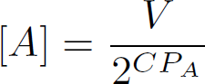
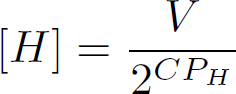
In the above equation. CP_A is the CT value of the gene of interest. CP_H, is the CT value of the household gene. Dividing the two obtained concentrations gives
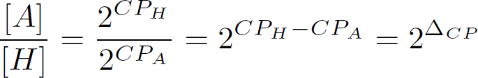
which is the first 'delta' in the delta-delta-CT method
Numerical Example 1
A has a CT value of 15.786H has a CT value of 18.875
DCT = 18.875-15.786
The concentration ratio is 8.51
This is an up-regulation of a factor 8.51 (against the household gene concentration)
Numerical Example 2
A has a CT value of 19.6H has a CT value of 12.4
DCT = 12.4-19.6 = -7.2
The concentration ratio is 0.068011
Which is a down regulation of a factor 147.03 (against the household gene concentration)
The concentrations produced by this normalization will be called relative concentration
Up/down regulations between celltypes
Often, one is interested in the up- or down-regulation from one cell type to the next. E.g: between a constitutive active cell line and an unmodified cell line. In that case, one must compare the relative concentrations between for instance the transgene and the wildtype cell type. This can be directly written down and expanded as follows
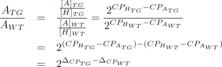
This means that to measure the up- or down- regulation between two cell types, thereby relying on a household gene, leads to 4 qPCR measurements (at the very least). If we are somewhat more scientific we need 2 measurements for the household genes, 2 measurements for the gene under investigation, 4 measurements for the different dilutions (1:1, 1:2, 1:5, 1:10 for instance), and three replicas, which altogether leads to 48 measurements.
Numerical example
Wildtype WT
A has a CT value of 15.786H has a CT value of 18.875
DCT = 18.875-15.786=3.089
Transgene TG
A has a CT value of 19.6H has a CT value of 12.4
DCT = 12.4-19.6 = -7.2
up- or down-regulation
DDCT = -7.2-3.089=-10.289WT/TG=0.000799286
or a down regulation by a factor 1251.12
A Common Layout
A common layout to deal with a number of genes and housholdgenes, while using triplicates and a dilution series is the followong
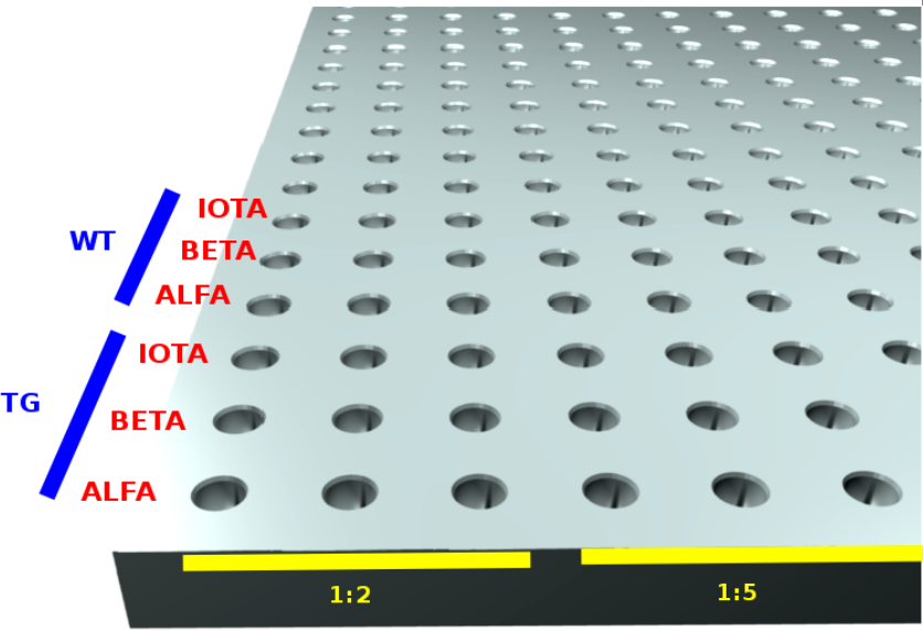
|
- Horizontally both the triplcates and dilutions are placed. E.g: 3 replicas of 1:2, then 3 replicas of 1:5 etcetera.
- vertically the householdgenes, genes and sample combinations are listed.
Software to calculate up/down regulations
Software to anlayze an up- down regulation experiment using qPCR is freely available at http://analysis.yellowcouch.org/qpcr/.| http://werner.yellowcouch.org/ werner@yellowcouch.org |  |