| Home | Papers | Reports | Projects | Code Fragments | Dissertations | Presentations | Posters | Proposals | Lectures given | Course notes |
|
|
BPM Measurement of Digital Audio by Means of Beat Graphs & Ray ShootingWerner Van Belle1* - werner@yellowcouch.org, werner.van.belle@gmail.com Abstract : In this paper we present a) a novel audio visualization technique, called beat-graphs and b) a fully automatic algorithm to measure the mean tempo of a song with a very high accuracy. The algorithm itself is an easy implementable offline search algorithm that looks for the tempo that best describes the song. For every investigated tempo, it steps through the song and compares the similarity of consecutive pieces of information (bass drum, a hi-hat, ...). Its accuracy is two times higher than other fully automatic techniques, including Fourier analysis, envelope-spectrum analysis and autocorrelation.
Keywords:
bpmdj meta data extraction tempo measurement beats per minute BPM measurement |
Table Of Contents
Introduction
Automatically measuring the tempo of a digital soundtrack is crucial for DJ-programs such as BpmDJ [1, 2], and other similar software. The ability to mix two (or more) pieces of music, depends almost entirely on the availability of correct tempo information. All too often this information must be manually supplied by the DJ. This results in inaccurate tempo descriptions, which are useless from a programming point of view [3]. Therefore we will investigate a technique to measure the tempo of a soundtrack accurately and automatically. In the upcoming discussion we assume that the audio fragments that need to be mixed have a fixed1 and initially unknown tempo.
The tempo of a soundtrack is immediately related to the length of a repetitive rhythm pattern encoded within the audio-fragment. This rhythm pattern itself can be virtually anything: a 4/4 dance rhythm, a 3/4 waltz, a tango, salsa or anything else. We assume that we have no information whatsoever about this rhythm pattern.
This paper is structured in four parts. First we elaborate on the required tempo accuracy. Second, we explain our beat graph visualization technique. This technique flows naturally into the the ray shooting algorithm, which is the third part. And last, we elaborate on our experiments and compare our technique with existing techniques.
Required Accuracy
Without accurate tempo information two songs will drift out of synchronization very quickly. This often results in a mix that degrades to chaos, which is not what we want. Therefore we must ask ourselves how accurately the tempo of a song should be measure to be useful. To express the required accuracy, we will calculate the maximum error on the tempo measurement to keep the synchronization drift after a certain timespan below a certain value.
We assume that the
tempo of the song is measured with an error ![]() .
If the exact tempo of the song is
.
If the exact tempo of the song is ![]() BPM then the measurement will
report
BPM then the measurement will
report ![]() BPM. Such a
wrong measurement leads to a drift
BPM. Such a
wrong measurement leads to a drift
![]() after a certain timespan
after a certain timespan ![]() . The timespan we consider,
is the time needed by the DJ to mix the songs. Typically this can
be 30'', 60'' or even up to 2 minutes if (s)he wants to alternate
between different songs. We will express the drift
. The timespan we consider,
is the time needed by the DJ to mix the songs. Typically this can
be 30'', 60'' or even up to 2 minutes if (s)he wants to alternate
between different songs. We will express the drift ![]() in
beats (at the given tempo), not in seconds. We chose not to use
absolute
time values because slow songs don't suffer as much from the same
absolute drift as fast songs. E.g, a drift of 25 ms is barely
noticeable
in slow songs (E.g, 70 BPM), while such a drift is very disturbing
for fast songs (E.g, 145 BPM). Therefore, we consider a maximum drift
of
in
beats (at the given tempo), not in seconds. We chose not to use
absolute
time values because slow songs don't suffer as much from the same
absolute drift as fast songs. E.g, a drift of 25 ms is barely
noticeable
in slow songs (E.g, 70 BPM), while such a drift is very disturbing
for fast songs (E.g, 145 BPM). Therefore, we consider a maximum drift
of ![]() beat, with
beat, with ![]() being the note-divisor. For instance,
we will calculate the required accuracy to keep the drift below
being the note-divisor. For instance,
we will calculate the required accuracy to keep the drift below ![]() ,
,
![]() and
and ![]() beat. Given the exact tempo
beat. Given the exact tempo ![]() (in BPM) and the measurement error
(in BPM) and the measurement error ![]() (in BPM), we can now
calculate the drift
(in BPM), we can now
calculate the drift ![]() (in beats) after timespan
(in beats) after timespan ![]() (in
seconds).
(in
seconds).
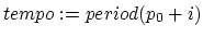
To do so, we must
first know how many beats are contained within the
timespan ![]() . Based on the
standard relation between period and frequency2, this is
. Based on the
standard relation between period and frequency2, this is
![]() beats.
Because the tempo is
measured with
an accuracy of
beats.
Because the tempo is
measured with
an accuracy of ![]() BPM, we get a
drift (expressed in beats)
of
BPM, we get a
drift (expressed in beats)
of
![]() .
To keep this drift below
.
To keep this drift below ![]() beat, we must keep
beat, we must keep ![]() .
Because
.
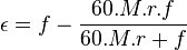
Because ![]() , we obtain a
required accuracy of
, we obtain a
required accuracy of

Equation 1 describes how accurately one song
should be measured to have a maximum possible drift of ![]() beats after a time of
beats after a time of ![]() seconds. In
practice, at least two songs
are needed to create a mix. If all involved songs are measured with
the same accuracy
seconds. In
practice, at least two songs
are needed to create a mix. If all involved songs are measured with
the same accuracy ![]() ,
then the maximum drift after
,
then the maximum drift after ![]() seconds
will be the sum of the maximum drifts of all involved songs. From
this, it becomes clear that we need to divide the required accuracy
by the number of songs. Table 2
gives an
overview of the required accuracies. As can be seen, an accuracy of
0.0313 BPM is essential, while an accuracy
of 0.0156 BPM
is comfortable.
seconds
will be the sum of the maximum drifts of all involved songs. From
this, it becomes clear that we need to divide the required accuracy
by the number of songs. Table 2
gives an
overview of the required accuracies. As can be seen, an accuracy of
0.0313 BPM is essential, while an accuracy
of 0.0156 BPM
is comfortable.
|
Beat Graphs
To explain our ray shooting technique we will first introduce the concept of beat-graphs. Not only can they help in manually measuring the tempo of a soundtrack, they also naturally extend to our ray-shooting technique.
| ||||
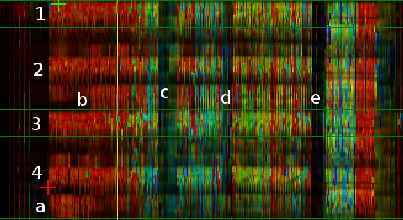
| Figure 1:Beat graphs of two songs. |
A beat graph visualizes an audio-stream (denoted as a series of samples
![]() ) under a certain period
) under a certain period ![]() . In the remainder of the text
we will assume that we are investigating an audio-fragment
. In the remainder of the text
we will assume that we are investigating an audio-fragment ![]() .
This fragment has a length of
.
This fragment has a length of ![]() samples and is sampled at a sampling
rate
samples and is sampled at a sampling
rate ![]() . If not specified
. If not specified ![]() will be considered to be a standard
of 44100 Hz. Given this notation, the beat graph
will be considered to be a standard
of 44100 Hz. Given this notation, the beat graph ![]() visualizes If
we have an audio fragment, denoted
visualizes If
we have an audio fragment, denoted ![]() , with a length of
, with a length of ![]() samples, It visualizes the function
samples, It visualizes the function
Horizontally, the measures are enumerated, while vertically the content
of one such a measure is visualized. The color of a pixel at position
![]() is given by the absolute strength of the signal at
time step
is given by the absolute strength of the signal at
time step ![]() . The value
. The value ![]() is the period of the rhythm pattern.
This typically contains 4 beats in a 4/4 key.
is the period of the rhythm pattern.
This typically contains 4 beats in a 4/4 key.
Picture 1 shows two beat graphs of Tandu and Posford [4, 5]. Reading a beat graph can best be done from top to bottom and left to right. For instance in the song Alien Pump [4] we see 4 distinct horizontal lines (numbers 1, 2, 3 and 4). These are the the 'beats' of the song. The top line covers all the beats on the first note in every measure, the second horizontal line covers all the beats at the second note within a measure and so on... The vertical white strokes that break the horizontal lines (C, D and E) are breaks within the music: passages without bass drum or another notable signal. Because the lines are distinctively horizontal we know that the period is correct. If the lines in the beat graph are slanted such as in Lsd [5]then the period (and thus the tempo) is slightly incorrect. In this case, the line is slanted upwards which means that the period is too short (the beat on the next vertical line comes before the beat on the current line), and this means that the tempo is a bit too high. By looking at the direction of the lines in a beat graph we can relate the actual tempo to the visualized tempo.
| ||||
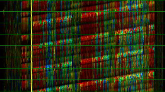
| Figure 2: Beat graphs of two songs. |
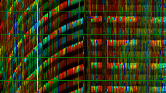
The beat graph not necessarily displays only straight lines. Two examples of this are given in figure 2. The first example is the song X-Files [6]. In the beginning the tempo line bends upward indicating that the song is brought down from a higher tempo. After a break the tempo remains constant. Another example is the song Anniversary Waltz [7] in which we clearly see a drummer who drifts around a target tempo.
Our visualization technique of beat graphs offers some important
advantages. First, the visualization function is very easy to
implement and can be calculated quickly. This is in stark contrast
with voice prints, which require extensive mathematical analysis and
offer no immediately useful tempo information. Secondly, the beat
graph contains rhythm information. From the viewpoint of the DJ, all
the necessary information is present. The temporal organization can be
recognized by looking at the picture. E.g, we can easily see how the
songs Alien Pump [4] contains beats at notes 1, 2, 3, 4 and
4![]() (position A
in the picture). After a while the extra beat at the end of a measure
is shifted forward in time by half a measure (position B). Similarly,
breaks and tempo changes can be observed (C, D and E). Third, as a
DJ-tool it offers a visualization that can be used to align the tempo
immediately. E.g, by drawing a line on the beat-graph such as done
in Lsd
[5], it is
possible to recalculate the graph with an adjusted period. Not only
will this introduce accurate tempo information, it also introduces the
information necessary to find the start of
a measure. This makes it easy to
accurately and quickly place cue-points.
(position A
in the picture). After a while the extra beat at the end of a measure
is shifted forward in time by half a measure (position B). Similarly,
breaks and tempo changes can be observed (C, D and E). Third, as a
DJ-tool it offers a visualization that can be used to align the tempo
immediately. E.g, by drawing a line on the beat-graph such as done
in Lsd
[5], it is
possible to recalculate the graph with an adjusted period. Not only
will this introduce accurate tempo information, it also introduces the
information necessary to find the start of
a measure. This makes it easy to
accurately and quickly place cue-points.
We will now further investigate how we can fully automatically line up the beat graph. If we are able to do so then we are able to calculate the tempo of a song automatically.
Ray Shooting
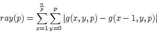
Beat graphs give us the possibility to visualize the tempo information within a song. We will now use this to search for the best possible visualization of the beat graph. An optimal visualization will give rise to as much 'horizontality' as possible. 'Horizontality' is measured by comparing every vertical slice (every measure) of the beat graph with the previous slice (the previous measure). Through accumulation of the differences between the consecutive slices we obtain a number that is large when little horizontality is present and small when a lot of horizontality is present. Formally, we measure
The use of the absolute value in the above equation is necessary to
accumulate the errors. If this would not be
present then a
mismatch between two measures at position ![]() could be compensated
for by a good match between two measures at another position
could be compensated
for by a good match between two measures at another position ![]() .
.
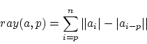
Equation 2 can be written more simply by expanding
![]() :
:
The problem we face now, is to find the period ![]() for which
for which ![]() is the smallest.
is the smallest. ![]() must be
located within a certain range, for
instance between the corresponding periods of 80 BPM and 160 BPM.
Once this period is found, we can convert it back to its tempo.
Converting
a period to BPM is done as follows.
must be
located within a certain range, for
instance between the corresponding periods of 80 BPM and 160 BPM.
Once this period is found, we can convert it back to its tempo.
Converting
a period to BPM is done as follows.
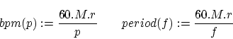
In the above conversion rules, ![]() denotes the number of beats within
the rhythm pattern. This typically depends on the key of the song.
For now, we will assume that every measure contains 4 beats, later
on we will come back to this and explain how this number can also
be measured automatically. Using the above equation we can define
the period range in which we are looking for the best match. We will
denoted this range
denotes the number of beats within
the rhythm pattern. This typically depends on the key of the song.
For now, we will assume that every measure contains 4 beats, later
on we will come back to this and explain how this number can also
be measured automatically. Using the above equation we can define
the period range in which we are looking for the best match. We will
denoted this range ![]() with
with ![]() the smallest
period
(thus the highest tempo) and
the smallest
period
(thus the highest tempo) and ![]() is the highest period (and thus
the lowest frequency). Given these two boundaries, we can calculate
the period of a song as follows
is the highest period (and thus
the lowest frequency). Given these two boundaries, we can calculate
the period of a song as follows
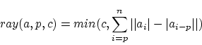
A possible optimization to this search process is the introduction of clipping values: When, during calculation of one of the rays, the current ray accumulates an error larger than the smallest ray until now (the clipping value) it can simply stops and returns the clipping value:
Because this ray function is limited to the computational complexity of the last best match, its calculation time can, as the number of scans increase, only decrease. The search algorithm can then be written down as
-
- for(
 ;
;  ;
;  )
)
if
Algorithmic Performance
The time needed to calculate the value of ![]() is
is ![]() .
Because
the period
.
Because
the period ![]() is often
neglectable small in comparison to the entire
length of a song, we omit it. Hence,
is often
neglectable small in comparison to the entire
length of a song, we omit it. Hence, ![]() takes
takes ![]() time to
finish. To find the best match in a certain tempo range by doing a
brute force search we need to shoot
time to
finish. To find the best match in a certain tempo range by doing a
brute force search we need to shoot ![]() rays. We will denote
the size of this window
rays. We will denote
the size of this window ![]() .
The resulting time estimate is accordingly
.
The resulting time estimate is accordingly
![]() . This performance estimate
is linear which might
look appealing, however, the size of the window is typically a very
large constant, so this performance estimate should be handled with
care. Nevertheless, the real strength of our approach comes from its
extremely high accuracy and its modular nature.
. This performance estimate
is linear which might
look appealing, however, the size of the window is typically a very
large constant, so this performance estimate should be handled with
care. Nevertheless, the real strength of our approach comes from its
extremely high accuracy and its modular nature.
Theoretical Accuracy
Our algorithm can verify any period above 0 and below ![]() .
This means that it can distinguish which one of two periods
.
This means that it can distinguish which one of two periods ![]() or
period
or
period ![]() is the best.
Therefore, we will calculate the accuracy
is the best.
Therefore, we will calculate the accuracy
![]() by measuring the smallest
distinguishable tempo. Given
a certain tempo, we will convert it to its period and then assume
that we have measured the period wrongly with the least possible error
of 1 sample. The two resulting periods are converted back to BPM's
and the differences between these two equals the theoretical
accuracy. Suppose the tempo of the song is
by measuring the smallest
distinguishable tempo. Given
a certain tempo, we will convert it to its period and then assume
that we have measured the period wrongly with the least possible error
of 1 sample. The two resulting periods are converted back to BPM's
and the differences between these two equals the theoretical
accuracy. Suppose the tempo of the song is ![]() , then the period of
this frequency is
, then the period of
this frequency is ![]() .
The closest distinguishable next period
is
.
The closest distinguishable next period
is ![]() . After
converting these two periods back to their
tempos we get
. After
converting these two periods back to their
tempos we get ![]() and thus an accuracy of
and thus an accuracy of
![]() .
Expansion of this expression results in
.
Expansion of this expression results in
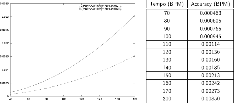
|
Table 3 presents an overview of the accuracies we might obtain with this technique. As can be seen, even the least accurate measurable tempo (170 BPM) can be distinguished with an accuracy of 0.00273, which is still 11 times more accurate than the required accuracy of 0.0313. For lower frequencies this even increases to 67.4 times better than the required accuracy ! It should be noted here that this is a theoretical accuracy. Later on we will experimentally validate the practical accuracy.
Selectivity
The algorithm as presented allows to verify the presence of one
frequency in ![]() . This opens
the possibilities to parallelize
the algorithm easily but also the possibility to actively search
for matching frequencies while neglecting large parts of the search
space. This of course requires a suitable search algorithm. In the
following section we will shed light on one search approach that has
proven to be very fast and still highly accurate.
. This opens
the possibilities to parallelize
the algorithm easily but also the possibility to actively search
for matching frequencies while neglecting large parts of the search
space. This of course requires a suitable search algorithm. In the
following section we will shed light on one search approach that has
proven to be very fast and still highly accurate.
Searching: Selective Descent
As explained in the previous section, verifying every possible frequency by doing a brute force search would take too much time. Nevertheless, the algorithm as presented here, allows the verification of single frequencies very accurately and quickly. This has lead to an algorithm that first does a quick scan of the entire frequency spectrum and then selects the most important peaks to investigate in further detail.
To skip large
chunks of the search space, we use an incremental approach.
First, the algorithm does a coarse grained scan that takes into account
'energy' blocks of information (let's say with a block size of ![]() ).
From the obtained results, it will decide which areas are the most
interesting to investigate in further detail. This is done by
calculating
the mean error of all measured positions. Everything below the mean
error will be investigated in the next step. We repeat this process
with a smaller block size of
).
From the obtained results, it will decide which areas are the most
interesting to investigate in further detail. This is done by
calculating
the mean error of all measured positions. Everything below the mean
error will be investigated in the next step. We repeat this process
with a smaller block size of ![]() until the block size becomes
1.
until the block size becomes
1.
The problem with
this approach is that it might very well overlook
steep dalls and consequently find and report a completely wrong
period/tempo.
To avoid this we will flatten the ![]() function by resampling
the input data to match the required block size.
function by resampling
the input data to match the required block size.
Resampling
To avoid a strongly oscillating ![]() function, which would make
a selective descent very difficult, we will, in every iteration step,
resample the audio stream to the correct frequency. This resampling
however is very delicate. Simply by taking the mean of the data within
a block, we will throw away valuable information. In fact, we will
throw everything away that cannot be represented at the given sampling
rate. E.g, if we have a block size of 1024 then the final sampling
rate will be 43 Hz. Such low sampling rates can only describe the
absolute low frequencies up to 21.5 Hz [8].
Please note here, that such a down sampling not only throws away
harmonics
(such as a down sampling from 44100 Hz to 22050 Hz would do), but
actually throws away entire pieces of useful information (like for
instance hi-hats). Such a sampling rate conversion is clearly not
what we are looking for. Therefore we have invented the following
resampling algorithm
function, which would make
a selective descent very difficult, we will, in every iteration step,
resample the audio stream to the correct frequency. This resampling
however is very delicate. Simply by taking the mean of the data within
a block, we will throw away valuable information. In fact, we will
throw everything away that cannot be represented at the given sampling
rate. E.g, if we have a block size of 1024 then the final sampling
rate will be 43 Hz. Such low sampling rates can only describe the
absolute low frequencies up to 21.5 Hz [8].
Please note here, that such a down sampling not only throws away
harmonics
(such as a down sampling from 44100 Hz to 22050 Hz would do), but
actually throws away entire pieces of useful information (like for
instance hi-hats). Such a sampling rate conversion is clearly not
what we are looking for. Therefore we have invented the following
resampling algorithm
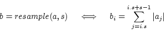
With every step,
the algorithm will first rescale the audio stream
by shrinking every block of ![]() sample to 1 sample. This is done
by taking the energy content of the block:
sample to 1 sample. This is done
by taking the energy content of the block:
As the caution reader may observe, we do not take the square of the
value ![]() as would be
necessary to correctly describe the energy
content of the block. The reason why we didn't is twofold. First
because
this approach is faster and keeps the values within
a reasonable bit range, hence remains accurate. Second, because we
are concerned with signals representing musical
content and
the spectrum of music already follows a power distribution.
as would be
necessary to correctly describe the energy
content of the block. The reason why we didn't is twofold. First
because
this approach is faster and keeps the values within
a reasonable bit range, hence remains accurate. Second, because we
are concerned with signals representing musical
content and
the spectrum of music already follows a power distribution.
Algorithm
With the knowledge how to resample the audio fragment and how to search
for the most prominent frequency, we can now write down the algorithm
in full detail. In the algorithm below ![]() is the number of beats
that are supposed to be in one measure.
is the number of beats
that are supposed to be in one measure.
![]() and
and
![]() (see equation 4).
The window size
(see equation 4).
The window size ![]() is given by
is given by ![]() . The resample function
is described in equation 6 and the
. The resample function
is described in equation 6 and the ![]() function
is described in equation 5.
function
is described in equation 5. ![]() is the number
of requested iterations. The maximum block size will then be
is the number
of requested iterations. The maximum block size will then be ![]() .
.
-
- 1.
![$matches:=[+\infty,\ldots\textrm{w times}\ldots,+\infty]$](img79.png)
2.
 resample(
  ,
,  )
) 3. for(
 ;
;  ;
;  )
) 4.
![$matches[j.2^{m}]:=$](img85.png) ray(
ray( ,
,  ,
,  )
) 5. for(
 ;
;  ;
;  )
) 6.
resample( ,  )
) 7. for(
;
 ; )
; ) 8. if
9.
![$match[j.2^{i}]:=$](img95.png) ray(,, )
ray(,, ) 10. for(
 , ;
, ;  ; )
; )
11. if
12.
 ray(
, ,
ray(
, ,  )
) 13. if
14.
15.

Performance
Estimating the performance of this algorithm is easy but requires
some explanation. Let us assume that we start with a block size of
![]() . This means that we will
iterate
. This means that we will
iterate ![]() steps.
steps.
The initial step,
with a block size of ![]() will result in
will result in ![]() rays to be shot. The cost to shoot one ray depends on the audio size.
After resampling this is
rays to be shot. The cost to shoot one ray depends on the audio size.
After resampling this is ![]() .
.
The following
steps, except for the last, are similar. However, here
it becomes difficult to estimate how many rays that will be shot,
because we take the mean error of the previous step and select only
the region that lies below the mean error. How large this area is,
is unknown. Therefore we will call the number of new rays divided
by the number of old rays the rest-factor ![]() . After one step,
we get
. After one step,
we get ![]() rays; after two steps this is
rays; after two steps this is
![]() and by
induction after
and by
induction after ![]() steps the number of rays becomes
steps the number of rays becomes ![]() .
Every ray, after resampling to a block size of
.
Every ray, after resampling to a block size of ![]() , takes
, takes ![]() time, hence the time estimation for every
time, hence the time estimation for every ![]() step is
step is
![]() .
We continue this process from
.
We continue this process from ![]() until
until ![]() .
.
The last step (![]() ) is similar, except that we
can do the ray shooting
it in half the expected time because we are looking for the minimum
and no longer for the mean error. This results in
) is similar, except that we
can do the ray shooting
it in half the expected time because we are looking for the minimum
and no longer for the mean error. This results in
![]()
The resampling cost
at every step is ![]() . After adding
all steps
together we obtain:
. After adding
all steps
together we obtain:
After some reductions, we obtain:
Depending on the factor of ![]() and
and
![]() we obtain different
performance
estimates. We have empirically measured the value of
we obtain different
performance
estimates. We have empirically measured the value of ![]() under a
window of [80 BPM:160 BPM]. We started our algorithm at a block
size of
under a
window of [80 BPM:160 BPM]. We started our algorithm at a block
size of ![]() and have
observed that the mean value of
and have
observed that the mean value of ![]() is
0.85. This results in an estimate of
is
0.85. This results in an estimate of ![]() . In practice, from
the possible 66150 rays to shoot we only needed to shoot 142,35 to
obtain the best match. So, we only searched 0.20313 % of the search
space before obtaining the correct answer. This is a speedup of about
246.18 times in comparison with the brute force search algorithm.
. In practice, from
the possible 66150 rays to shoot we only needed to shoot 142,35 to
obtain the best match. So, we only searched 0.20313 % of the search
space before obtaining the correct answer. This is a speedup of about
246.18 times in comparison with the brute force search algorithm.
Experiments
Setup
We have implemented this algorithm as a BPM counter for the DJ program
BpmDj [1]. The
program can measure the tempo of
.MP3 and .OGG files. It is written in C++ and runs under Linux. The
program can be downloaded from http://bpmdj.sourceforge.net/.
The parameters the algorithm currently uses are: ![]() ,
, ![]() ,
,
![]() . Of course these can be modified when
necessary.
The algorithm starts iterating at
. Of course these can be modified when
necessary.
The algorithm starts iterating at ![]() and stops at
and stops at ![]() because
a higher accuracy is simply not needed.
because
a higher accuracy is simply not needed.
| ||||
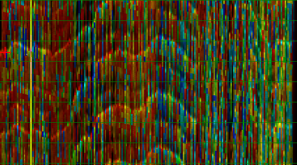
| Figure 3:Tempo scanning two songs. |
Figure 3 shows the output it produces for two songs. Every color presents the results of one scanning iteration. The first scan is colored green, the last scan is colored red. The horizontal colored lines represent the position of the mean values for that scan. As can be seen, by using the mean value, quickly large parts of the search space are omitted.
Comparing against related work
To compare the accuracy of our technique with other measurement techniques, we also inserted two well-known BPM-measurement techniques into BpmDj. The first technique does a Fourier analysis of the audio envelope in order to find the most prominent frequency. The second techniques calculates the power density spectrum of the audio sample, which happens to be the same as the autocorrelation function. Techniques that are not fully automatically have been omitted. Hence, we excluded techniques that make use of a database describing possible rythms [11]. Below we briefly describe some other techniques.
Peak Detectors
Peak detectors [12]make use of Fourier analysis
or specially tuned digital filters to spike at the occurrence of bass
drums (frequencies between 2 and 100 Hz), hi-hats (above 8000 Hz)
or other repetitive sounds. By analyzing the distance between the
different spikes, they might be able to obtain the tempo. The problem
with such techniques is that they are inherent inaccurate, and not
only requires detailed fine tuning of the filter-bank but afterwards
still require a comprehension phase of the involved rhythm . Their
inaccuracy comes from the problem that low frequencies (encoding a
bass drum for instance) have a large period, which makes it difficult
to position the sound accurately. In other words, the Fourier analysis
will spike somewhere around the actual
position of the beat,
thereby making the algorithm inherent inaccurate. The
second
problem of peak detectors involves the difficulties of designing a
set of peak-responses that will work for all songs. E.g, some songs
have a hard and short bass-drum with a lot of body while other song
have a muffled slowly decaying bass-drum. Tuning the algorithm such
that it can detect correctly the important sounds in almost all songs
can be difficult. Finally, the last problem of peak detectors is that
they often have no notion of the involved rhythm. E.g,
a song
with a drum line with beats at position 1, 2, 3, 4 and ![]() are notoriously difficult to understand because the last spike at
position
are notoriously difficult to understand because the last spike at
position ![]() will
seriously lower the mean time between
the different beats. This can be remedied through using a knowledge
base of standard rhythms.
will
seriously lower the mean time between
the different beats. This can be remedied through using a knowledge
base of standard rhythms.
In comparison with peak detectors our technique is clearly superior because it is a) much easier to implement, b) does not require a comprehension phase and c) is much more accurate.
Fourier Analysis of the Energy Envelope
This technique obtains the energy envelope of the audio sample and
will then transform it to its frequency representation. The most
prominent
frequency can be immediately related to the tempo of the audio fragment
[13, 14]. From a performance
point of view this techniques
are much better than the algorithm we presented. Especially if one
makes use of the Goertzel algorithm [15]. The accuracy
of these techniques can be theoretically as good as our technique,
assuming that one takes a window-size that is large enough. E.g, to
have an accuracy of 0.078 BPM at a sampling rate of 44100 Hz one needs
at least a window size of ![]() ,
which is an audio-fragment of 12' 40''. When such a window-size is not
available (because the audio-fragment
is not as long), the envelope should be zero-padded up to the required
length [15].
,
which is an audio-fragment of 12' 40''. When such a window-size is not
available (because the audio-fragment
is not as long), the envelope should be zero-padded up to the required
length [15].
Autocorrelation
At first sight, our algorithm might seem similar to autocorrelation [15]because we compare the song with itself at different distances. However, this
is only a superficial similarity. To understand
this we point out that autocorrelation for a discrete audio signal
![]() is defined as
is defined as
![]() . As can be
seen, the comparison between different slices is done by multiplying
the different values. In our algorithm we only measure the distance
between the absolute values, so there is no clear direct correspondence
between ray shooting and autocorrelation. Nevertheless autocorrelation
has been applied to obtain the mean tempo of an audio fragment. The
computation of
. As can be
seen, the comparison between different slices is done by multiplying
the different values. In our algorithm we only measure the distance
between the absolute values, so there is no clear direct correspondence
between ray shooting and autocorrelation. Nevertheless autocorrelation
has been applied to obtain the mean tempo of an audio fragment. The
computation of ![]() can be done
using quickly using two Fourier
transforms. The process takes 3 steps. First the audio-fragment is
transformed to its frequency-domain, then every sample is replaced
with its squared norm and finally a backward Fourier transform is
done. Formally,
can be done
using quickly using two Fourier
transforms. The process takes 3 steps. First the audio-fragment is
transformed to its frequency-domain, then every sample is replaced
with its squared norm and finally a backward Fourier transform is
done. Formally, ![]() .
.
Experiment
The experiment consisted of a selection of 150 techno songs. The tempo of each song has been manually measured through aligning their beat graphs. All songs had a tempo between 80 BPM and 160 BPM. Of them 7 had a drifting tempo. In these songs we have manually selected the largest straight part (such as done for the song X-Files [6]). Afterwards, we have run the BPM counter on all the songs again. For every song the counter reported the measurements using different techniques and the time necessary to obtain this value. The machine on which we did the tests was a Dell Optiplex GX1, 600 MHz running Debian GNU/Linux. The counter has been compiled with the Gnu C Compiler version 3.3.2 with maximum optimization, but without machine specific instructions.
Results & Discussion
Harmonics
The song Tainted Love [10] (see
picture 3) is interesting because it
shows 4
distinct spikes in the ray-shoot analysis. Every spike is a multiple
of each other. In fact, the ![]() spike is the actual tempo with
a measured period of 4 beats, which is a correlation between beat
1 and beat 5. The
spike is the actual tempo with
a measured period of 4 beats, which is a correlation between beat
1 and beat 5. The ![]() spike occurs when the algorithm correlates
between the 1st and the
spike occurs when the algorithm correlates
between the 1st and the ![]() beat, hence calculates a tempo with
measures of 5 beats, while it expects to find only 4 beats in a
measure.
This results in a tempo of 114.5. The
beat, hence calculates a tempo with
measures of 5 beats, while it expects to find only 4 beats in a
measure.
This results in a tempo of 114.5. The ![]() spike is similar but
now a correlation between the
spike is similar but
now a correlation between the ![]() and the
and the ![]() beat occurs.
The first spike is a correlation between the
beat occurs.
The first spike is a correlation between the ![]() beat and the
beat and the
![]() beat. We have these distinct
spikes because the song is
relatively empty and monotone.
beat. We have these distinct
spikes because the song is
relatively empty and monotone.
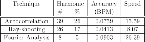
All techniques have a problem with estimating how many beats are located within one rhythmic pattern. When a tempo is reported that is a multiple of the required tempo we call it an harmonic.
Results
|
The results of our experiment can be downloaded from http://bpmdj.sourceforge.net/bpmcompare.html or seen in the appendix.
As expected the
results contained a number of wrongly reported errors
due to harmonics. These have been detected and eliminated by simply
multiplying the reported period by ![]() ,
, ![]() or
or ![]() . The
autocorrelation technique reported an harmonic
tempo in 26% of the cases, the ray-shooting technique in 17 % and
the Fourier analysis in 5 %. Clearly the Fourier analysis is superior
with respect to the problem of harmonics.
. The
autocorrelation technique reported an harmonic
tempo in 26% of the cases, the ray-shooting technique in 17 % and
the Fourier analysis in 5 %. Clearly the Fourier analysis is superior
with respect to the problem of harmonics.
However, with respect to the accuracy of the measurement, our ray-shooting technique is best. It measures the mean tempo with an accuracy of 0.0413. From which we can conclude that our algorithm has a practical accuracy of 0.0340 BPM, which is close to the required accuracy of 0.0313. The autocorrelation technique has an accuracy of 0.0759 BPM. The Fourier analysis has an accuracy of 0.0903 BPM. The latter is consistent with reported accuracies. If we look at the speed of our algorithm then it is clearly outperformed. Both the autocorrelation and Fourier analysis are between 2 and 4 time as fast as the autocorrelation technique.
Key + Period = Tempo = Key/Period
Our ray shooting technique finds the period of an unknown repetitive rhythm pattern. As observed it might sometimes report an harmonic of the actual tempo. This happens because we have always assumed that every rhythm pattern contains 4 beats (see equation 4). In practice this is not always the case for two reasons.
First, because not
all songs are written in a 4/4 key, we can easily
have a different number of beats within the rhythm pattern. E.g, a
rhythm pattern with a length of 2 seconds, in a 4/4 key will have
4 beats, hence a tempo of
![]() , which
is a tempo of 120 BPM. On the other hand, if the rhythm pattern is
written in a 3/4 key, these 2 seconds will only have 3 beats, which
leads to a tempo of 90 BPM.
, which
is a tempo of 120 BPM. On the other hand, if the rhythm pattern is
written in a 3/4 key, these 2 seconds will only have 3 beats, which
leads to a tempo of 90 BPM.
The second reason why we cannot assume that every rhythm pattern will always contain 4 beats is that our algorithm might sometimes find rhythm patterns that have a period that is factor different from the actual pattern. This happens mostly when the rhythm pattern itself is monotone and the song shows little rhythmic variation. (As we have explained for the song ``Tainted Love'')
As observed from
our results, the Fourier analysis has little problems
with harmonics, however it is less accurate than our technique.
Therefore,
a combination of both techniques might yield a high accuracy without
too much problems of harmonics. Specifically, we could easily modify
the algorithm such that it would in its first iteration fill the ![]() array with the spectrum of the envelope. Formally, line 4 of our
algorithm becomes
array with the spectrum of the envelope. Formally, line 4 of our
algorithm becomes ![]() .
.
Conclusion
In this paper we have introduced our visualization technique, called beat graphs. A beat graph shows the structure of the music under a certain tempo. It shows rhythmic information, covering where breaks and beats are positioned and tempo information. Beat graphs can be quickly drawn and are a valuable tool for the digital DJ, because they can also be used as a fingerprint of songs.
Based on these beat graphs, we have developed an offline algorithm to determine the tempo of a song fully automatically. The algorithm works by shooting rays through the digital audio and checking the similarities between consecutive slices within the audio. To speed up the process of finding the best matching ray, we presented an optimized search algorithm that must only search 0.2% of the entire search space.
The BPM counter
works fully correct in 82% of the cases.
The
other 17% are correctly measured but
report a tempo that is
an harmonic of the actual tempo. The remaining one percent is measured
incorrectly . The accuracy of the measurement is 0.0340 BPM, which
is enough to keep the drift of two songs below ![]() beat
after 30'' (or to keep the drift below
beat
after 30'' (or to keep the drift below ![]() beat after
60''). Aside from being very accurate, our algorithm is also
insensitive
to breaks and gaps in the audio stream. The algorithm is 8.33 faster
than real time on a 600 MHz Dell Optiplex, without making use of
processor
specific features.
beat after
60''). Aside from being very accurate, our algorithm is also
insensitive
to breaks and gaps in the audio stream. The algorithm is 8.33 faster
than real time on a 600 MHz Dell Optiplex, without making use of
processor
specific features.
Full Result Listing
The table below contains 150 songs, all which have been measured a) manually using beat-graphs, b) autmatically using our rayshooting technique, c) automatically using autocorrelation and d) automatically using a fourier analysis of the audio enveloppe. For every song we have compared the measured tempo against the actual tempo. In a number of cases this tempo is a multiple of the actual tempo beacuse the algorithm measures a period which contains a wrong number of actual beats. E.g, 5 beats, 7 beats, 3 beats and so on. Based on these harmonics we have rescaled the measurement and compared the reported tempo with the measured tempo. This denotes the measurement error. Only for the fourier analysis of the enveloppe we have avoided in doing so (this is reported in the colum: 'Before'). We did this because the fourier analysis measure the most prominent frequency, not the best matchin period. As such are the harmonics of this technique often much more wrong than the harmonics of the two other techniques. As such, fixing the measurement of the fourier technique might give a wrong impression. Therefore the before colum only takes into account the ones that were acutally measured correctly.
| Measurement Error (BPM) |
|||||||||||
|
Measured Period
|
Harmonic |
After fixing
harmonics |
Before | ||||||||
| Title | Manual | Ray | Cor | Env | Rayshoot | Correl | Envelop | Rayshoot | Correl | Envelop | Envelop |
| MonsterHit_2[Hallucinogen] | 132300 | 132296 | 82675 | 66182 | 1 | 0.63 | 0.5 | 0 | 0.01 | 0.04 | |
| AndTheDayTurnedToNight_7[Hallucinogen] | 128288 | 112268 | 112259 | 89777 | 0.88 | 0.88 | 0.75 | 0.01 | 0.01 | 5.92 | |
| TheHerbGarden[Hallucinogen] | 109120 | 109120 | 109128 | 109120 | 1 | 1 | 1 | 0 | 0.01 | 0 | 0 |
| God[]2 | 106264 | 106264 | 106259 | 106184 | 1 | 1 | 1 | 0 | 0 | 0.08 | 0.08 |
| StillDreaming(AnythingCanHappen)[AstralProjection] | 105944 | 105960 | 105964 | 70640 | 1 | 1 | 0.63 | 0.02 | 0.02 | 6.26 | |
| After1000Years[InfectedMushroom] | 88204 | 88180 | 88188 | 88185 | 1 | 1 | 1 | 0.03 | 0.02 | 0.03 | 0.03 |
| ElCielo[Spacefish] | 86136 | 85948 | 86899 | 86147 | 1 | 1 | 1 | 0.27 | 1.08 | 0.02 | 0.02 |
| NextToNothing[] | 84888 | 84888 | 84887 | 75488 | 1 | 1 | 0.88 | 0 | 0 | 2 | |
| Skydiving[ManWithNoName] | 82672 | 82624 | 82627 | 66182 | 1 | 1 | 0.75 | 0.07 | 0.07 | 8.08 | |
| 3MinuteWarning[YumYum]2 | 79572 | 79548 | 79556 | 79607 | 1 | 1 | 1 | 0.04 | 0.03 | 0.06 | 0.06 |
| Voyager3{PaulOakenFold_7}[Prana] | 79048 | 118548 | 118555 | 79137 | 1.5 | 1.5 | 1 | 0.03 | 0.02 | 0.15 | 0.15 |
| ElectronicUncertainty[Psychaos] | 78900 | 78896 | 78891 | 78951 | 1 | 1 | 1 | 0.01 | 0.02 | 0.09 | 0.09 |
| FromFullmoonToSunrise[] | 78484 | 78484 | 78475 | 78489 | 1 | 1 | 1 | 0 | 0.02 | 0.01 | 0.01 |
| Foxglove[Shakta] | 78476 | 78480 | 78475 | 78306 | 1 | 1 | 1 | 0.01 | 0 | 0.29 | 0.29 |
| Shakti[Shakta] | 78468 | 78468 | 78467 | 78489 | 1 | 1 | 1 | 0 | 0 | 0.04 | 0.04 |
| DawnChorus[ManWithNoName] | 78392 | 97984 | 97980 | 78398 | 1.25 | 1.25 | 1 | 0.01 | 0.01 | 0.01 | 0.01 |
| CowsBlues[DenshiDanshi] | 78368 | 78368 | 78367 | 78398 | 1 | 1 | 1 | 0 | 0 | 0.05 | 0.05 |
| KumbaMeta[DjCosmix&Etnica] | 78064 | 78064 | 78063 | 78033 | 1 | 1 | 1 | 0 | 0 | 0.05 | 0.05 |
| Teleport{PaulOakenfold_4}[ManWithNoName] | 77944 | 116916 | 116911 | 77852 | 1.5 | 1.5 | 1 | 0 | 0.01 | 0.16 | 0.16 |
| Vavoom[ManWithNoName] | 77828 | 77832 | 116743 | 77852 | 1 | 1.5 | 1 | 0.01 | 0 | 0.04 | 0.04 |
| Possession[TheDominatrix] | 77828 | 77824 | 77823 | 77852 | 1 | 1 | 1 | 0.01 | 0.01 | 0.04 | 0.04 |
| 1998{MattDarey}[BinaryFinary] | 77824 | 77804 | 77815 | 77672 | 1 | 1 | 1 | 0.03 | 0.02 | 0.27 | 0.27 |
| AncientForest[Sungod]2 | 77820 | 77824 | 77823 | 77852 | 1 | 1 | 1 | 0.01 | 0.01 | 0.06 | 0.06 |
| LunarJuice{Hallucinogen}[SlinkyWizard]2 | 77816 | 77816 | 77815 | 77852 | 1 | 1 | 1 | 0 | 0 | 0.06 | 0.06 |
| MorphicResonance[Cosmosis] | 77776 | 77776 | 77775 | 77762 | 1 | 1 | 1 | 0 | 0 | 0.02 | 0.02 |
| TittyTwister[Viper2] | 77332 | 77344 | 77332 | 77314 | 1 | 1 | 1 | 0.02 | 0 | 0.03 | 0.03 |
| Cambodia[Prometheus] | 77260 | 77236 | 77255 | 77225 | 1 | 1 | 1 | 0.04 | 0.01 | 0.06 | 0.06 |
| InvisibleCities{Tristan}[BlackSun] | 77256 | 96572 | 96571 | 77403 | 1.25 | 1.25 | 1 | 0 | 0 | 0.26 | 0.26 |
| OpenTheSky[Transparent] | 77256 | 77252 | 77252 | 77225 | 1 | 1 | 1 | 0.01 | 0.01 | 0.05 | 0.05 |
| Bongraiders[Necton] | 77244 | 77252 | 77252 | 77225 | 1 | 1 | 1 | 0.01 | 0.01 | 0.03 | 0.03 |
| BinaryFinary[BinaryFinary] | 76940 | 76944 | 96883 | 76871 | 1 | 1.25 | 1 | 0.01 | 1.01 | 0.12 | 0.12 |
| AuroraBorealis[AstralProjection] | 76776 | 76812 | 76004 | 76783 | 1 | 1 | 1 | 0.06 | 1.4 | 0.01 | 0.01 |
| LiquidSunrise[AstralProjection]2 | 76772 | 76760 | 76776 | 76783 | 1 | 1 | 1 | 0.02 | 0.01 | 0.02 | 0.02 |
| AllBecauseOfYou{Minesweeper}[UniversalStateOfMind] | 76760 | 76760 | 76764 | 76783 | 1 | 1 | 1 | 0 | 0.01 | 0.04 | 0.04 |
| Tranceport[PaulOakenfold] | 76708 | 76704 | 76687 | 76783 | 1 | 1 | 1 | 0.01 | 0.04 | 0.13 | 0.13 |
| LowCommotion[ManWithNoName] | 76692 | 95860 | 95852 | 76695 | 1.25 | 1.25 | 1 | 0.01 | 0.02 | 0.01 | 0.01 |
| VisionsOfNasca[AstralProjection]3 | 76692 | 115060 | 115056 | 76695 | 1.5 | 1.5 | 1 | 0.03 | 0.02 | 0.01 | 0.01 |
| VisionsOfNasca[AstralProjection] | 76688 | 115060 | 115056 | 76695 | 1.5 | 1.5 | 1 | 0.03 | 0.03 | 0.01 | 0.01 |
| PsychedelicTrance[GoaRaume] | 76688 | 76680 | 76683 | 76695 | 1 | 1 | 1 | 0.01 | 0.01 | 0.01 | 0.01 |
| Spawn[EatStatic] | 76164 | 95200 | 95200 | 75829 | 1.25 | 1.25 | 1 | 0.01 | 0.01 | 0.61 | 0.61 |
| EyeTripping[ForceOfNature] | 76164 | 76160 | 76136 | 75915 | 1 | 1 | 1 | 0.01 | 0.05 | 0.46 | 0.46 |
| Fly[AstralProjection]3 | 76156 | 76168 | 76172 | 76173 | 1 | 1 | 1 | 0.02 | 0.03 | 0.03 | 0.03 |
| TimeBeganWithTheUniverse{TheEndOfTime}[AstralProjection] | 75944 | 75964 | 75963 | 75915 | 1 | 1 | 1 | 0.04 | 0.03 | 0.05 | 0.05 |
| TimeBeganWithTheUniverse[AstralProjection]2 | 75944 | 75964 | 75963 | 75915 | 1 | 1 | 1 | 0.04 | 0.03 | 0.05 | 0.05 |
| Joy[Endora] | 75812 | 75820 | 75819 | 75829 | 1 | 1 | 1 | 0.01 | 0.01 | 0.03 | 0.03 |
| Twisted[InfectedMushroom] | 75700 | 75704 | 75703 | 75915 | 1 | 1 | 1 | 0.01 | 0.01 | 0.4 | 0.4 |
| WalkOnTheMoon[TheAntidote] | 75684 | 75684 | 75696 | 75658 | 1 | 1 | 1 | 0 | 0.02 | 0.05 | 0.05 |
| Utopia[AstralProjection] | 75680 | 75700 | 75699 | 75658 | 1 | 1 | 1 | 0.04 | 0.04 | 0.04 | 0.04 |
| TheFeelings[AstralProjection] | 75676 | 75664 | 75667 | 75915 | 1 | 1 | 1 | 0.02 | 0.02 | 0.44 | 0.44 |
| MaianDream[AstralProjection]2 | 75676 | 75800 | 113195 | 75658 | 1 | 1.5 | 1 | 0.23 | 0.39 | 0.03 | 0.03 |
| TajMahal[Microworld] | 75676 | 75704 | 75679 | 75658 | 1 | 1 | 1 | 0.05 | 0.01 | 0.03 | 0.03 |
| TranceDance[AstralProjection]3 | 75676 | 75680 | 113511 | 75658 | 1 | 1.5 | 1 | 0.01 | 0 | 0.03 | 0.03 |
| DayDreamOne[TheDr] | 75676 | 94592 | 94587 | 75658 | 1.25 | 1.25 | 1 | 0 | 0.01 | 0.03 | 0.03 |
| Unknown1[AstralProjection]2 | 75668 | 75668 | 75671 | 75658 | 1 | 1 | 1 | 0 | 0.01 | 0.02 | 0.02 |
| InNovation{originalmix}[AstralProjection]2 | 75668 | 75884 | 75892 | 75658 | 1 | 1 | 1 | 0.4 | 0.41 | 0.02 | 0.02 |
| MagneticActivity[MFG] | 75664 | 75656 | 75664 | 75658 | 1 | 1 | 1 | 0.01 | 0 | 0.01 | 0.01 |
| Contact[EatStatic] | 75656 | 75596 | 113496 | 75573 | 1 | 1.5 | 1 | 0.11 | 0.01 | 0.15 | 0.15 |
| XFile[Chakra&EdiMis] | 75632 | 75624 | 113455 | 75573 | 1 | 1.5 | 1 | 0.01 | 0.01 | 0.11 | 0.11 |
| Kaguya[SunProject] | 75608 | 75592 | 75595 | 75658 | 1 | 1 | 1 | 0.03 | 0.02 | 0.09 | 0.09 |
| GetInTrance[DjMaryJane] | 75608 | 75636 | 75615 | 75573 | 1 | 1 | 1 | 0.05 | 0.01 | 0.06 | 0.06 |
| Soothsayer{LysurgeonWarningMix}[Hallucinogen] | 75604 | 75596 | 75595 | 75573 | 1 | 1 | 1 | 0.01 | 0.02 | 0.06 | 0.06 |
| SeratoninSunrise{Mvo}[ManWithNoName] | 75604 | 75592 | 75607 | 75573 | 1 | 1 | 1 | 0.02 | 0.01 | 0.06 | 0.06 |
| Upgrade[AphidMoon] | 75600 | 75600 | 113400 | 75573 | 1 | 1.5 | 1 | 0 | 0 | 0.05 | 0.05 |
| Cyanid[Colorbox]2 | 75596 | 75596 | 75595 | 75573 | 1 | 1 | 1 | 0 | 0 | 0.04 | 0.04 |
| GodIsADj{AstralProjection}[Faithless]3 | 75592 | 75832 | 75824 | 75573 | 1 | 1 | 1 | 0.44 | 0.43 | 0.04 | 0.04 |
| Amen[AstralProjection] | 75584 | 76200 | 75559 | 75573 | 1 | 1 | 1 | 1.13 | 0.05 | 0.02 | 0.02 |
| PsychedelicIndioCrystal[MultiFreeman] | 75584 | 75576 | 75575 | 100764 | 1 | 1 | 1.38 | 0.01 | 0.02 | 4.4 | |
| SmallMoves[InfectedMushroom] | 75584 | 75580 | 75583 | 75573 | 1 | 1 | 1 | 0.01 | 0 | 0.02 | 0.02 |
| TheUltimateSin[Cosmosis] | 75560 | 75556 | 75559 | 75573 | 1 | 1 | 1 | 0.01 | 0 | 0.02 | 0.02 |
| Diablo[Luminus] | 75536 | 75536 | 75535 | 75573 | 1 | 1 | 1 | 0 | 0 | 0.07 | 0.07 |
| Cor[GreenNunsOfTheRevolution] | 75508 | 75500 | 75503 | 75488 | 1 | 1 | 1 | 0.01 | 0.01 | 0.04 | 0.04 |
| Laet[Fol] | 75472 | 75472 | 75471 | 75488 | 1 | 1 | 1 | 0 | 0 | 0.03 | 0.03 |
| MindEruption[SubSequence] | 75144 | 75140 | 75140 | 75149 | 1 | 1 | 1 | 0.01 | 0.01 | 0.01 | 0.01 |
| OverTheMoon[Phreaky] | 75136 | 75140 | 75140 | 75149 | 1 | 1 | 1 | 0.01 | 0.01 | 0.02 | 0.02 |
| Ionised{PaulOakenfold}[AstralProjection]2 | 75116 | 75112 | 75115 | 75065 | 1 | 1 | 1 | 0.01 | 0 | 0.1 | 0.1 |
| Spacewalk[Shivasidpao] | 75064 | 75044 | 75060 | 75065 | 1 | 1 | 1 | 0.04 | 0.01 | 0 | 0 |
| DanceOfWitches{Video}[SunProject] | 74860 | 74868 | 74859 | 74898 | 1 | 1 | 1 | 0.02 | 0 | 0.07 | 0.07 |
| Track05[] | 74628 | 74632 | 74631 | 74400 | 1 | 1 | 1 | 0.01 | 0.01 | 0.43 | 0.43 |
| FlyingIntoAStar[AstralProjection] | 74608 | 74660 | 74647 | 74565 | 1 | 1 | 1 | 0.1 | 0.07 | 0.08 | 0.08 |
| KeyboardWidow[Psychaos] | 74608 | 93268 | 93247 | 74648 | 1.25 | 1.25 | 1 | 0.01 | 0.02 | 0.08 | 0.08 |
| PeopleCanFly{AlienProject}[AstralProjection] | 74540 | 74540 | 74540 | 74482 | 1 | 1 | 1 | 0 | 0 | 0.11 | 0.11 |
| DroppedOut[Zirkin&Bonky] | 74536 | 130436 | 75123 | 74482 | 1.75 | 1 | 1 | 0 | 1.11 | 0.1 | 0.1 |
| HFEnergy{Heaven}[AminateFx] | 74532 | 74532 | 74532 | 74565 | 1 | 1 | 1 | 0 | 0 | 0.06 | 0.06 |
| TimeBeganWithTheUniverse[AstralProjection]5 | 74532 | 74492 | 74500 | 74565 | 1 | 1 | 1 | 0.08 | 0.06 | 0.06 | 0.06 |
| FreeReturn[Alienated] | 74156 | 74324 | 130051 | 74400 | 1 | 1.75 | 1 | 0.32 | 0.31 | 0.47 | 0.47 |
| InnerReflexion[AviAlgranatiAndBansi] | 74096 | 74096 | 74096 | 74071 | 1 | 1 | 1 | 0 | 0 | 0.05 | 0.05 |
| CosmicAscension[AstralProjection] | 74084 | 73992 | 74007 | 74071 | 1 | 1 | 1 | 0.18 | 0.15 | 0.03 | 0.03 |
| FullMoonDancer[Dreamscape]2 | 74024 | 74024 | 74024 | 73989 | 1 | 1 | 1 | 0 | 0 | 0.07 | 0.07 |
| InvisibleContact[PigsInSpace] | 74004 | 111016 | 111023 | 73989 | 1.5 | 1.5 | 1 | 0.01 | 0.02 | 0.03 | 0.03 |
| GiftOfTheGods[Cosmosis]2 | 73992 | 73996 | 73996 | 73989 | 1 | 1 | 1 | 0.01 | 0.01 | 0.01 | 0.01 |
| FluoroNeuroSponge_7[Hallucinogen]3 | 73764 | 129084 | 129080 | 73746 | 1.75 | 1.75 | 1 | 0 | 0.01 | 0.04 | 0.04 |
| LetThereBeLight[AstralProjection] | 73572 | 73592 | 73583 | 73584 | 1 | 1 | 1 | 0.04 | 0.02 | 0.02 | 0.02 |
| ObsceneNutshell[LostChamber] | 73568 | 73572 | 73572 | 73584 | 1 | 1 | 1 | 0.01 | 0.01 | 0.03 | 0.03 |
| ElectricBlue[AstralProjection] | 73500 | 73500 | 110252 | 73503 | 1 | 1.5 | 1 | 0 | 0 | 0.01 | 0.01 |
| PsychedeliaJunglistia[CypherO] | 73496 | 110220 | 73456 | 73343 | 1.5 | 1 | 1 | 0.03 | 0.08 | 0.3 | 0.3 |
| LifeOnMars[AstralProjection]2 | 73496 | 73252 | 74215 | 73503 | 1 | 1 | 1 | 0.48 | 1.4 | 0.01 | 0.01 |
| Nilaya[AstralProjection]3 | 73488 | 73484 | 73480 | 72865 | 1 | 1 | 1 | 0.01 | 0.02 | 1.23 | 1.23 |
| OmegaSunset[Mantra]2 | 73464 | 73444 | 110223 | 73423 | 1 | 1.5 | 1 | 0.04 | 0.04 | 0.08 | 0.08 |
| Eternal[Epik] | 73220 | 73220 | 73224 | 73262 | 1 | 1 | 1 | 0 | 0.01 | 0.08 | 0.08 |
| Paradise[AstralProjection]2 | 73176 | 73176 | 73175 | 73103 | 1 | 1 | 1 | 0 | 0 | 0.14 | 0.14 |
| MadLane[Psychaos] | 73076 | 73076 | 73080 | 73103 | 1 | 1 | 1 | 0 | 0.01 | 0.05 | 0.05 |
| Tatra[Antartica] | 73068 | 109592 | 109587 | 120266 | 1.5 | 1.5 | 1.63 | 0.01 | 0.02 | 1.84 | |
| OnlineInformation[ElectricUniverse] | 73064 | 91320 | 73088 | 73023 | 1.25 | 1 | 1 | 0.02 | 0.05 | 0.08 | 0.08 |
| AbsoluteZero_6[TotalEclipse]2 | 73064 | 73064 | 73067 | 73023 | 1 | 1 | 1 | 0 | 0.01 | 0.08 | 0.08 |
| Ganesh[Sheyba] | 73052 | 91312 | 91311 | 73023 | 1.25 | 1.25 | 1 | 0 | 0.01 | 0.06 | 0.06 |
| SpiritualAntiseptic[Hallucinogen] | 73004 | 73004 | 72999 | 73023 | 1 | 1 | 1 | 0 | 0.01 | 0.04 | 0.04 |
| Freakuences[ElectricUniverse] | 73004 | 109520 | 109500 | 73023 | 1.5 | 1.5 | 1 | 0.02 | 0.01 | 0.04 | 0.04 |
| ShivaDevotional[Shivasidpao] | 73004 | 73004 | 72999 | 73023 | 1 | 1 | 1 | 0 | 0.01 | 0.04 | 0.04 |
| TechnoPrisoners[Phreaky]2 | 73004 | 127796 | 72528 | 73023 | 1.75 | 1 | 1 | 0.04 | 0.95 | 0.04 | 0.04 |
| Deliverance[Butler&Wistler] | 72996 | 109492 | 109491 | 73023 | 1.5 | 1.5 | 1 | 0 | 0 | 0.05 | 0.05 |
| AstralPancake[Hallucinogen] | 72996 | 72996 | 72995 | 73023 | 1 | 1 | 1 | 0 | 0 | 0.05 | 0.05 |
| Viper[Viper] | 72992 | 72952 | 109467 | 73023 | 1 | 1.5 | 1 | 0.08 | 0.03 | 0.06 | 0.06 |
| TransparentFuture[AstralProjection]2 | 72988 | 72988 | 72999 | 73023 | 1 | 1 | 1 | 0 | 0.02 | 0.07 | 0.07 |
| IWannaExpand[Cwhite] | 72976 | 72976 | 127671 | 72944 | 1 | 1.75 | 1 | 0 | 0.04 | 0.06 | 0.06 |
| GetOut[DarkEntity] | 72972 | 72732 | 72752 | 72944 | 1 | 1 | 1 | 0.48 | 0.44 | 0.06 | 0.06 |
| LSDance[Psysex] | 72964 | 72916 | 72948 | 72944 | 1 | 1 | 1 | 0.1 | 0.03 | 0.04 | 0.04 |
| OuterBreath[Aztec] | 72924 | 127608 | 127603 | 72944 | 1.75 | 1.75 | 1 | 0.01 | 0.02 | 0.04 | 0.04 |
| Shamanix_5[Hallucinogen]2 | 72608 | 72604 | 72603 | 72628 | 1 | 1 | 1 | 0.01 | 0.01 | 0.04 | 0.04 |
| Shamanix[Hallucinogen] | 72608 | 72604 | 72603 | 72628 | 1 | 1 | 1 | 0.01 | 0.01 | 0.04 | 0.04 |
| Inspiration[Mfg] | 72564 | 72564 | 72564 | 72550 | 1 | 1 | 1 | 0 | 0 | 0.03 | 0.03 |
| Androids[TechnoSommy] | 72564 | 72568 | 72568 | 72550 | 1 | 1 | 1 | 0.01 | 0.01 | 0.03 | 0.03 |
| HypnoTwist[Tripster] | 72556 | 72588 | 108840 | 72550 | 1 | 1.5 | 1 | 0.06 | 0.01 | 0.01 | 0.01 |
| Schizophonic[XIS] | 72512 | 72500 | 108752 | 72471 | 1 | 1.5 | 1 | 0.02 | 0.02 | 0.08 | 0.08 |
| TheWorldOfTheAcidDealer[TheInfinityProject] | 72496 | 72492 | 72312 | 72471 | 1 | 1 | 1 | 0.01 | 0.37 | 0.05 | 0.05 |
| Vertige2[GoaGil] | 72480 | 90584 | 90603 | 72628 | 1.25 | 1.25 | 1 | 0.03 | 0 | 0.3 | 0.3 |
| Zwork[SunProject] | 72460 | 72472 | 126736 | 72471 | 1 | 1.75 | 1 | 0.02 | 0.08 | 0.02 | 0.02 |
| Exposed[CatOnMushrooms] | 72084 | 72088 | 72088 | 72082 | 1 | 1 | 1 | 0.01 | 0.01 | 0 | 0 |
| TouchTheSon[Sundog]2 | 72004 | 72000 | 71996 | 72005 | 1 | 1 | 1 | 0.01 | 0.02 | 0 | 0 |
| SonicChemist[Psychaos] | 71996 | 71988 | 71992 | 72005 | 1 | 1 | 1 | 0.02 | 0.01 | 0.02 | 0.02 |
| AcidKiller{Hallucinogen}[InfectedMushroomXerox] | 71968 | 71964 | 71963 | 72005 | 1 | 1 | 1 | 0.01 | 0.01 | 0.08 | 0.08 |
| TurnOnTuneIn[Cosmosis] | 71960 | 71964 | 71960 | 71928 | 1 | 1 | 1 | 0.01 | 0 | 0.07 | 0.07 |
| SnarlingBlackMabel_6[Hallucinogen] | 71904 | 71904 | 71904 | 71928 | 1 | 1 | 1 | 0 | 0 | 0.05 | 0.05 |
| Lust{ArtOfTranceRemix}[] | 71580 | 71600 | 71592 | 71620 | 1 | 1 | 1 | 0.04 | 0.02 | 0.08 | 0.08 |
| MidnightZombie[SunProject] | 71508 | 71508 | 71508 | 71468 | 1 | 1 | 1 | 0 | 0 | 0.08 | 0.08 |
| ThreeBorgfour[Shivasidpao] | 71504 | 89364 | 89367 | 71468 | 1.25 | 1.25 | 1 | 0.03 | 0.02 | 0.07 | 0.07 |
| TheFirstTouer[CosmicNavigators] | 71476 | 71496 | 71484 | 71468 | 1 | 1 | 1 | 0.04 | 0.02 | 0.02 | 0.02 |
| KitchenSync[Synchro] | 71212 | 106824 | 71211 | 126620 | 1.5 | 1 | 1.75 | 0.01 | 0 | 2.35 | |
| FastForwardTheFuture{HallucinogenMix}[ZodiacYouth]3 | 70800 | 70800 | 70800 | 70789 | 1 | 1 | 1 | 0 | 0 | 0.02 | 0.02 |
| VirtualTerminalEnergised_1[TotalEclipse]2 | 70632 | 70628 | 70627 | 70640 | 1 | 1 | 1 | 0.01 | 0.01 | 0.02 | 0.02 |
| TheNeuroDancer[Shakta] | 70620 | 70616 | 105920 | 70640 | 1 | 1.5 | 1 | 0.01 | 0.01 | 0.04 | 0.04 |
| Micronesia[ShaktaMoonweed] | 70616 | 70616 | 88275 | 70640 | 1 | 1.25 | 1 | 0 | 0.01 | 0.05 | 0.05 |
| Spawn[Beast] | 70572 | 123496 | 123496 | 70566 | 1.75 | 1.75 | 1 | 0.01 | 0.01 | 0.01 | 0.01 |
| Chapachoolka[SunProject] | 70560 | 70548 | 70552 | 70492 | 1 | 1 | 1 | 0.03 | 0.02 | 0.14 | 0.14 |
| 380Volt[SunProject] | 70524 | 70516 | 70515 | 70492 | 1 | 1 | 1 | 0.02 | 0.02 | 0.07 | 0.07 |
| SpiritualTranceTrack6[GoaGil] | 69236 | 69236 | 69235 | 69255 | 1 | 1 | 1 | 0 | 0 | 0.04 | 0.04 |
| Diffusion[Shidapu] | 69104 | 69104 | 69103 | 69255 | 1 | 1 | 1 | 0 | 0 | 0.33 | 0.33 |
| PsychicPhenomenon[Ultrabeat]2 | 68724 | 68720 | 68715 | 68688 | 1 | 1 | 1 | 0.01 | 0.02 | 0.08 | 0.08 |
| Hybrid{TheInfinityProject}[EatStatic] | 68308 | 68312 | 68311 | 68200 | 1 | 1 | 1 | 0.01 | 0.01 | 0.25 | 0.25 |
| Part1[Psilocybin] | 67916 | 67928 | 67940 | 67923 | 1 | 1 | 1 | 0.03 | 0.06 | 0.02 | 0.02 |
| BeneathAnIndianSky[RoyAquarius]2 | 67480 | 67480 | 67479 | 67243 | 1 | 1 | 1 | 0 | 0 | 0.55 | 0.55 |
| Measurement
Error |
124 | 111 | 142 | 0.0413 | 0.0759 | 0.2914 | 0.0903 | ||||
| Variance |
0.0148 | 0.0562 | 1.0952 | 0.0215 | |||||||
Bibliography
| 1. | BpmDj: Free DJ Tools for Linux Werner Van Belle 1999-2010 http://bpmdj.yellowcouch.org/ |
| 2. | Beatforce Computer DJ-ing System John Beuving 25 September 2001 http://beatforce.berlios.de/ |
| 3. | Hang the DJ: Automatic sequencing and seamless mixing of dance-music tracks Dave Cliff Technical report, Digital Media Systyems Departement, Hewlett-Pacakrd Laboratories, Bristol BS34 8QZ England, June 2000 |
| 4. | Alien Pump Tandu Distance To Goa 6, Label: Distance (Substance) Records, 1997 |
| 5. | LSD SImon Posford (Hallucinogen) Dragonfly Records, 1995 |
| 6. | X-Files Chakra & Edimis Retro 10 Years of Israeli Trance, Label: Phonokol, 2001 |
| 7. | Anniversary Walz Status Quo Label: Castle Music, 1990 |
| 8. | Certain Topics in Telegraph Transmission Theory Harry Nyquist AIEE Trans., 47:617-644, 1928 |
| 9. | Rolling On Chrome Aphrodelics remicex by Kruder & Dorfmeister Studio K7, 1990 |
| 10. | Tainted Love Soft Cell Warner, May 1996 |
| 11. | Music understanding at the beat level: Real-time beat tracking for audio signals M. Goto, Y. Muraoka Readings in Computational Auditory Scene Analysis, 1997 |
| 12. | Apparatus for detecting the number of beats Yamada, Kimura, Tomohiko, Funada, Takeaki, Inoshita, and Gen US Patent Nr 5,614,687, December 1995 |
| 13. | Estimation of tempo, micro time and time signature from percussive music Christian Uhle, Jürgen Herre Proceedings of the 6th International Conference on Digital Audio Effects (DAFX-03), London, UK, September 2003 |
| 14. | Tempo and beat analysis of acoustic musical signals Scheirer, Eric D Journal of the Acoustical Society of America, 103-1:588, January 1998 |
| 15. | Discrete-Time Signal Processing Alan V. Oppenheim, Ronald W. Schafer, John R. Buck Signal Processing Series. Prentice Hall, 1989 |
Footnotes
- ...fixed1
- Admittedly, not all songs fall in this category, nevertheless we can safely make this assumption because we are only interested in the audio fragments that are to be mixed. Also, very few DJ's will mix two songs when one of the tempos changes too much.
- ... frequency2
- BPM and Hz are both units of frequency. To convert BPM to Hz we
simply
multiply or divide by 60:
 and
and  . If we have a frequency
specified
in BPM then we can obtain the time between two beats in msecs with
. If we have a frequency
specified
in BPM then we can obtain the time between two beats in msecs with
 .
.
| http://werner.yellowcouch.org/ werner@yellowcouch.org |  |