| Home | Papers | Reports | Projects | Code Fragments | Dissertations | Presentations | Posters | Proposals | Lectures given | Course notes |
|
|
Fast Tempo Measurement: a 6000x sped-up autodifferencer.Werner Van Belle1 - werner@yellowcouch.org, werner.van.belle@gmail.com Abstract : The autodifference is often used to measure the tempo of music. This technique requires quadratic time, with one parameter being the tempo range under investigation and the second being the songlength. In this paper we describe a number of improvements to this analysis technique to reduce the number of required calculations with a factor of 6272. We also report on a solution for the problem of autodifferencebiases and finally we explain a new solution to resolve tempo harmonic for 4/4 rhythms.
Keywords:
Tempo Analysis, Fast Tempo Measurement, Tempo Harmonics, 4/4 Rhythm, BPM measurement |
Table Of Contents
Introduction
Analyzing the tempo of music is important for DJ applications because it they need it to mix two songs. It also forms a first step in meta-data extraction. Such extraction can lead to rhythm patterns, composition information, time signatures and potentially other useful information.
Analyzing the tempo of music has been a remarkably hard problem up to date. A number of techniques exist to estimate the tempo of music. Among them are the spectrum analysis of the energy envelope, autocorrelation of the full song, or off the energy envelope, auto-differencing of the energy envelope [1]or autodifferencing the actual data [2]. In all these cases only about 75% of the songs is measured correctly. All other songs tend to be reported as multiples of the actual tempo. E.g: if the song is in reality a 120 BPM 4/4 song, then it might also be reported as a 96 BPM song (if the algorithm believes that one measure contains 4 beats while it actually spanned 5 beats). On the other hand, if the algorithm believes that only 3 beats cover a measure, while still believing that each measurement contains 4 beats then the tempo will be reported as 160 BPM.
In 2010 I made a number of improvements such that on a test-set of 2130 songs, 98% of all songs were correctly measured, if we allowed tempo harmonics that were the double of halve of the actual tempo. The algorithm was thus allowed to report 45 BPM, instead of 90. It could however not report 120 (which would be the 1.3 harmonic). This reduced the problem from a multi-class classification problem to a binary classification problem, which is sufficiently useful for DJ applications. In particular, when a DJ application wants to mix one song (e.g: 120 BPM) with another song at 60 BPM, it should not speed up the second song a factor 2, but assume that the second one was really 120 BPM. One could assume now that this argumentation could also be used to deal with all harmonics, including 5/4, 3/4, 7/4, 3/6, etc, but in that case the harmonics tend to be too close to one another to help the program.
In this paper, we report on some new improvements on tempo analysis, especially in the area of bias-reduction, speed, and harmonic resolving for 4/4 rhythms. But before we delve into these improvements it is maybe wise to briefly summarize what the autodifference is and on what type of data we have been working.
Autodifferencing
The autodifference, given a certain measure length (the period), is defined as:
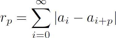
The autodifference plots horizontally the period (p) and vertically the value of r_p.
| ||||
| Two (biased) autodiffrence plots of the same song. Left the tempo against the autodifference is set out. Right the period against the autodifference. |
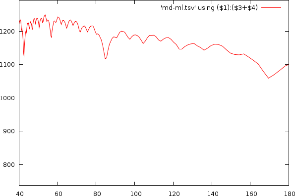
The positions where the autodifference has a low value are the potential tempo candidates.
Improvement #1: Energy location in the average song
A first area where we were able to improve the speed of autodifferencing is by not calculating the autodifference of the entire song, but merely of a suitable large and correctly positioned fragment. Instead of measuring the full 8 minutes, we can get away with measuring only 1 minute.
The main question here is of course: which minute do we take. We could for instance choose the start of the song (which is not a good idea, most songs have much less energy in the beginning than anywhere else). Or, an intuitive approach, would be to select the middle of the song, which would work. However, relative many long techno songs have breaks in the middle, which would produce less value for the time we spent in such an area.
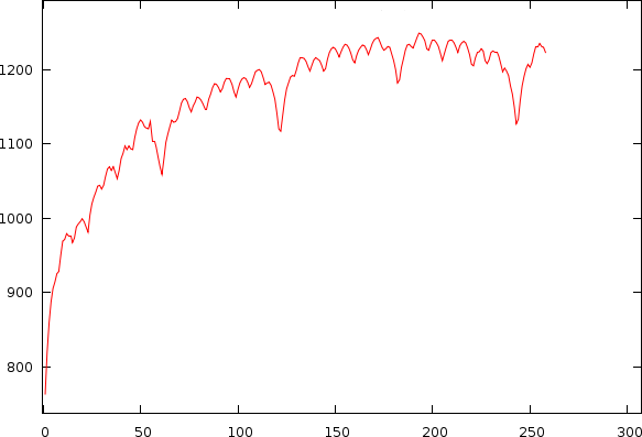
 Around 3600 songs were analyzed
and their energy measured at various positions. Each songs
energy was normalized to a position betwen 0 and 1 and an energy
maximum of 1. All these profiles were averaged together.
Around 3600 songs were analyzed
and their energy measured at various positions. Each songs
energy was normalized to a position betwen 0 and 1 and an energy
maximum of 1. All these profiles were averaged together.
|
To understand which area we should use to analyze the tempo we looked into the average energy against songposition (in %) and found that the most energy is locate at 90%. When one thinks about it, it makes sense. After the big finale, nothing comes. Nothing is to be said or to be done. Throw out the song and find the next one.
This means, that the most valuable minute is to be found at the 90% position of the song and then go back 1 minute. This area will provide the most useful information to analyze the tempo. On average this leads to a speedup of 8
Improvement #2: Selecting a proper blocksize
Another speedup was achieved by working with the energy content of a song instead of the raw samples. This reduced the sound size by a factor of 32. So instead of looking at each individual sample, we would combine 32 of them together by taking the absolute value of the left and right channels together. This technique is comparable to the algorithm presented earlier [1], where we attempted to extract melody lines. It is also comparable to the first technique [2] in which we iteratively refined the block size. However, we found that the accuracy at a certain block size drops substantially, while the analysis time goes up. That is normal since at a certain block size we start to measure individual samples and we might get locked in a certain position through phase interactions, which in themselves have nothing to do with what our ears perceive, and certainly not with where we would locate that energy.
 Horizontally the test-blocksize
is set out. Vertically we present the accuracy and the % correct
tempo-harmonics. We did this for two dataset. A minmal techno
set (around 360 songs) and a full dataset of 3600 songs. As can
be seen, the best tempo harmonics performance is found under a
blocksize of 32. And in the all set there also appears little
gain of lowering the blocksize to improve on accuracy.
Horizontally the test-blocksize
is set out. Vertically we present the accuracy and the % correct
tempo-harmonics. We did this for two dataset. A minmal techno
set (around 360 songs) and a full dataset of 3600 songs. As can
be seen, the best tempo harmonics performance is found under a
blocksize of 32. And in the all set there also appears little
gain of lowering the blocksize to improve on accuracy.
|
Conclusion: a block size of 32 samples provides the best tempo
accuracy.
Speedup: x 32
Improvement #3: Avoid biases
The bias in the autodifference plot is the logarithmic shape one sees in the period vs mismatch plot. As we observed previously, this bias is unique for each song, so it cannot be averaged across many songs and then subtracted. We attempted around 14 different techniques to get rid of the bias, while at the same time being unable to explain where it comes from. 'A form of coherent noise' was the best we could do to describe it. I recently finally figured out where it comes from:
A first (obvious) aspect to this bias is that we expect interdependency within the autodifference plot: Suppose I measure a low autodifference at lag X, then at twice that lag we would also expect a low autodifference. But that is not sufficient to explain the bias in itself.
| ||||||||
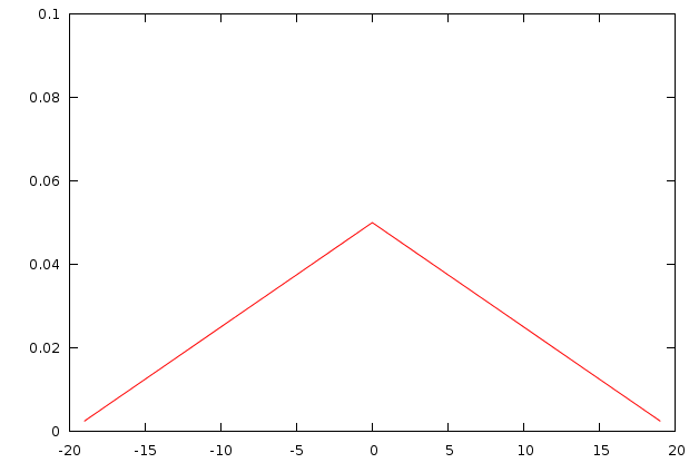
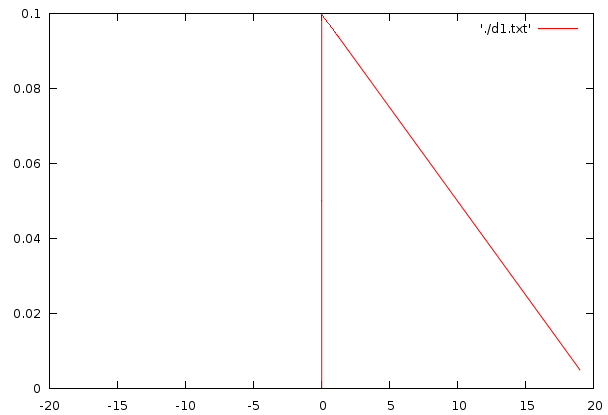
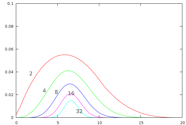
| This image demonstrates how the variance of the energy and the number of measurements affects the reported autodifference. The first plot illustrates the energy distribution. In general each position on the sampled ray has an engery between 90 and 110. The difference of two consecutive points is thus distributed according to the second figure, with potential negeative enegry differences. After taking the absolute vlae of this, we obtain a stricltyy positive value and a distribution according to figure 3. We then add multiple of such measurements (and divide the result by the number of additions performed), which is visibialized for 2,4,8,16, and 32 additions. This series of distributions shows that the number of autodifference sampling points changes the expected outcome. This illustrates two things: 1) the variance oif the signal affects the autodifference, 2) the number of sampling points has an unexpected effect on the measured autodifference |
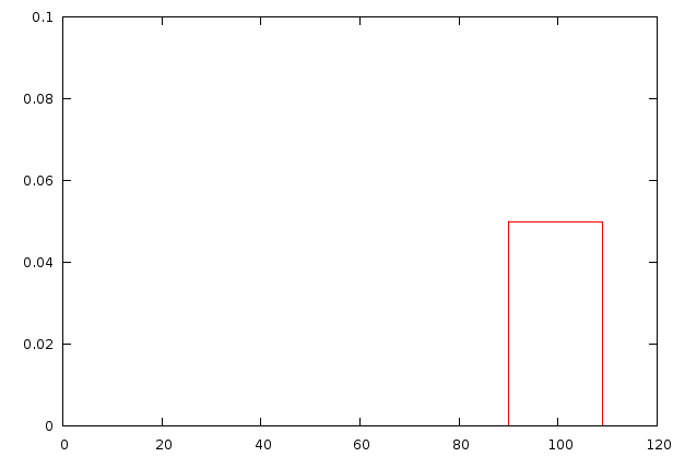
As to understand the bias we can create a small simulation in which we have a signal that should have an autodifference of 0 (each position in the song has value 100), but to which we added a uniform noise, which results in a song where each position contains a value between 90 and 110. If we simulate such a setup through a simply statistical distribution (see figure), we find two interesting properties
- The noise does not cancel out and is added to the signal, this is due to the absolute value we employ.
- The impact of noise does not increase linearly if we add more samples. It appears to be incrementing in a logarithmic fashion.
Of course, noise is something we get for free when dealing with audio. it can be there because the artist didn't follow strict metronome. It can be there because other frequencies cross the bassdrum we are investigating. It can be there because there because of phaseinteractions.
However, the results also indicate that if we use the same number of sampling points for each investigated lag, the effects of noise will be the same in all bins, which leads to a solution to this problem. Namely: don't oversample, use the same number of sampling points for each investigated measure length. Aside from removing the bias, this approach also speeds up the algorithm, since we won't compare that many positions anymore.
Conclusion: the autodifference plot is dependent on the variance of the signal and on the number of times the signal has been summed together.
Improvement #4: Turn the algorithm upside down
The normal algorithm [2], takes an audio block, resamples it, and then for each potential tempo, measures the similarity between each position and its next measure. This unnecessary, it is sufficient to select a number of sampling points. This leads to a dramatic speedup since, instead of scanning 78553 positions (this is the number of potential locations in 57 seconds at a block size of 32 and a minimum rhythm of 90 BPM), we can get away with randomly sampling around 3200 positions. An extra advantage of this is that we can choose to limit this technique in time.
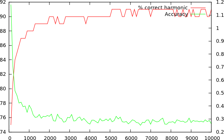 Horizontal
the number of sampling points is shown. The red line shows how many %
of the measurments reported the correct harmonic (from 74 to 92
%). The green line shows how accurate those measurements are
(expressed in % from 0.2% up to 1.2%)
Horizontal
the number of sampling points is shown. The red line shows how many %
of the measurments reported the correct harmonic (from 74 to 92
%). The green line shows how accurate those measurements are
(expressed in % from 0.2% up to 1.2%)
|
Conclusion: instead of investigating every possible position in
a song, it is sufficient to sample 3200 positions for each
investigated tempo
Speedup: ~24.
Improvement #5: A deharmonization strategy
The problem with a collection of peaks is that they are all equally viable options if we look at them individually. However, when we deal with 4/4 rhythms there are some tricks that we can apply to merge multiple peaks onto fewer peaks.
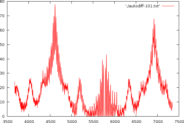
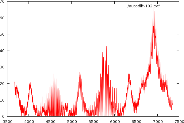
Peak Detection
Although, the author of this paper hates peak detection (see [3, 4] to get an impression on how much he hates it), it turns out that it is actually a viable method to speed up this particular algorithm. The peak detector works by first finding the maximum value in the dataset. From there on the flanks are removed by always subtracting the 'minimum so far'. So if we start at a maximum of 123, and the neighboring data point is 75, then we will subtract 75 from the 75, leaving 0. The neighbor of 75 , which in this example is 80, will undergo a lowering of 75 as well (that is the minimum value we saw so far), resulting in a value of 15. All these masses can be added together, leading to a position, mass and height for each peak.
| ||||||||
| A serie of images showing the extraction of peaks and their neighbouring masses. |
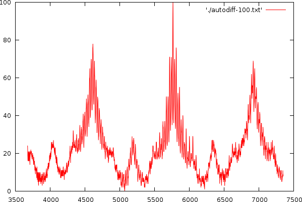
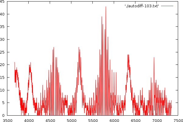
This leads to a series of peaks, their height, and position. As long as the peak is above 30% of the global maximum, we consider it a viable one. Otherwise we stop the algorithm. If a peak is within 5% of an earlier peak we do not add it and we also do not reposition that peak, otherwise we loose quite a bit of accuracy in the algorithm.
Asigning a harmonic to a detected repetition
This technique tries to determine for each found peak, what type of harmonic it is. Whether we found a repetition at 3/4th of a measure, or whether we found a repetition at 5/4 of a measure. Based on that we then try to generate an overall picture of the likelihood that a certain tempo is correct.
The possibility to assign a harmonic to a certain peak is based on the fact that the various possible interpretations of each peak, will lead to different relative position for the neighboring peaks. Let us first assume that we have a peak at position 120 BPM, which was measured correctly after 4 beats. In a simple rhythm we will also find a repetition after 3 beats, so we expect a peak at position 160 BPM (which is 120*4/3). We also expect to find a peak if we autodifference the track on 5 beats. That leads to another secondary peak at 96 BPM (120*4/5). So, as soon as we find a peak at position 1, and also its neighboring peaks at position 1.3333 and 0.8, then we have an indication that it was a 4 beat long harmonic. Now, if we are dealing with a peak that was measured after 3 beats, at e.g: 120 BPM, then we expect also a peak after 4 beats, which brings us at position 90 BPM (120*3/4). Further, we could also find a peak after 2 beats, or at position 180 BPM (120*3/2). Expressing this relatively, if the peak we investigate is a 3 beat long harmonic, then we expect to find neighboring peaks at position 1.5 and 0.75. This distinction in neighboring peaks is of course valuable.
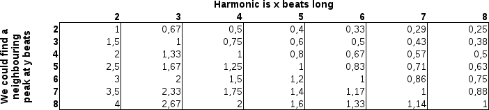 Crosstable of all possible multipliers and dividers
|
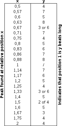
Of course there is an entire range of possible dividers and multipliers. Our assumption that we have a 3,4,5,6 beat harmonic, together with its potential neighboring peaks can initially best be expressed as a crosstable (see above). This table is then inverted so that we obtain a mapping from 'relative position of neighbor' to 'indicates harmonic X'.
| ||||
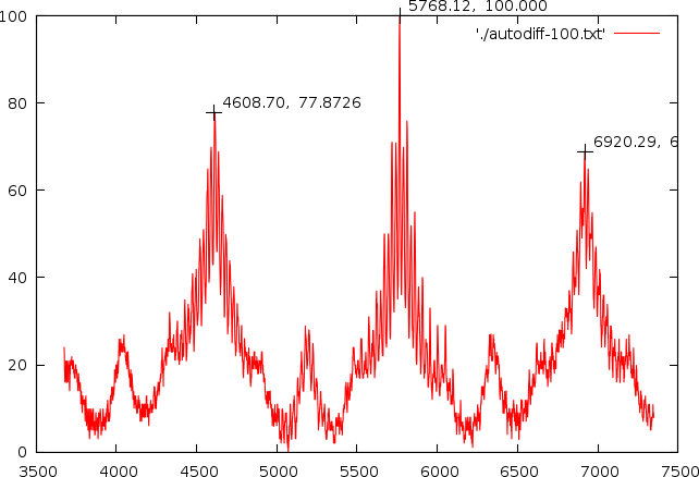
| The potential relative peak positions and their meaning, when such peak is present. In the right picture we see a number of peaks and for demonstrative purposes we will assess each of the peaks. Peak 1 is at position 4608.7. Its first neighbor is at relative position 1.2515 (5768.12/4608.7), indicating that this peak is a harmonic with 4 beats. Its second neighbor is at relative position 1.5, indication harmonic 2 or 4. Peak 2 is at position 5768.12. It first neighbor is at relative position 0.7989, indicating a 5 harmonic. It second neighbor is at relative position 1.1997, indicating harmonic 5 as well. Peak 3 has also two neighbors at relative positions 0.6659 (indicating 3 or 6) and 0.8335, indicating harmonic 6. |
Combining all guesses for all peaks
For each peak we obtain a number of guesses. So, when n peaks are present we have n*(n-1) values to deal with. In practice this doesn't form a bottleneck. The only thing worth mentioning is how the combination is performed: Instead of producing a fixed value (harmonic 3 or 4), we accumulate indications for both of them. For instance if a relative position 0.775 is present, then we will put value 0.5 in harmonic bins 4 and 5, since it is between those two. Once all peaks are aggregated it is straightforward to recompute the target tempo for a 4beat harmonic.
That process is done for all peaks and in general leads to only 2 potential result tempos, both of which can be weighted again given the total accumulated evidence for that tempo'.
Technically it might be necessary here to allow the reporting of tempos that are substantially higher or lower than what is an acceptable range. It is only once the tempos have been reported that division or multiplication by 2 becomes appropriate. If we place such rescaling into the search range too early, it messes up the entire algorithm
Results
The data collection
The data collection we worked with consisted of 3700 songs, including psychedelic trance, techno, minimal techno, dub and popular music. All songs have been manually annotated with the correct tempo by means of beatgraphs. If the visualized graph is horizontal then the tempo was correct. If the tempo was somewhat incorrect, we modified the beatgraph such that it would be horizontal. As such, we knew the tempo be exactly for all songs, and also makes it possible later on to report on the accuracy of the technique.
Sensitivity
To understand the accurate working of our algorithm we tested it on our dataset and ordered the results in bins of 5BPM, according to their actual tempo and then counted the number of reported harmonics in each bin.
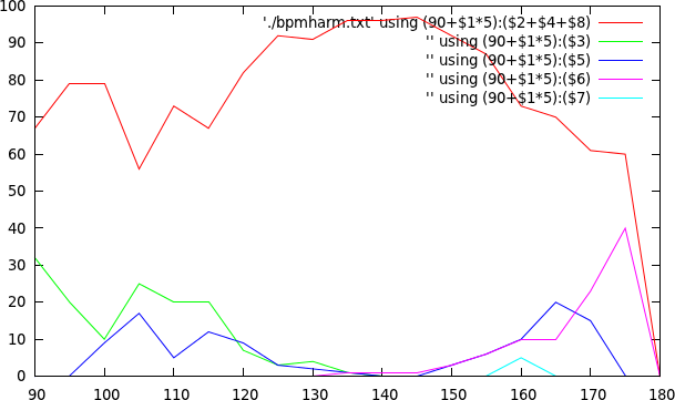 Horizontally the excat tempo is
set out and for each of these tempos we report how many times a
certain tempo harmonic has been reported. Red: correct tempo harmonic,
double or qudruple. Green: measured as 4/3 of the actual tempo. Blue:
measured as 5/4th of the actual tempo. Purple: measured as 6/4th of
the actual tempo. Turquoise: measured as 7/4th of the actual tempo.
Horizontally the excat tempo is
set out and for each of these tempos we report how many times a
certain tempo harmonic has been reported. Red: correct tempo harmonic,
double or qudruple. Green: measured as 4/3 of the actual tempo. Blue:
measured as 5/4th of the actual tempo. Purple: measured as 6/4th of
the actual tempo. Turquoise: measured as 7/4th of the actual tempo.
|
The presented algorithm is somewhat sensitive around the border cases. This is due to the fact that a tempo of 96 its harmonic (which might be present) has not been measured. So all in all there is potentially more material present to force a 5/3 harmonic since there is no balance on the right side.
Conclusions
We presented a number of optimizations to speed up autodifferencing by a factor of 6272.
- Select an audio block from the song from 90% - 60s to 90%. This is the area that contains, on average, the highest energy. (*8)
- It is sufficient to sample around 3200 positions in the audio block to have a sensible autodifference plot. (*24.5)
- Biases can be avoided by having the same number of sample points for each potential lag
- The preferred block size is 16 or 32 samples long. (*32)
- A technique to assign a harmonic number to extracted peaks has been presented as well as a method to combine multiple peak indications in a limited number of tempo candidates.
In case of 4/4 rhythms a complicated peak detection and tempo-harmonic assignment algorithm can provide sensible hints to select the correct tempo harmonic.
Future Work
- The use of zero crossings as a similarity measure, or the use of local sensitive hashes to compare energy blocks might provide some valuable input into the algorithm.
- We did not yet test the border cases against larger window sizes
- The sampling approach might make it possible to deal with changing tempos by allowing a certain drift at each position.
References
| 1. | Biasremoval from BPM Counters and an argument for the use of Measures per Minute instead of Beats per Minute Van Belle Werner Signal Processing; YellowCouch; July 2010 http://werner.yellowcouch.org/Papers/bpm10/ |
| 2. | BPM Measurement of Digital Audio by Means of Beat Graphs & Ray Shooting Werner Van Belle December 2000 http://werner.yellowcouch.org/Papers/bpm04/ |
| 3. | Correlation analysis of two-dimensional gel electrophoretic protein patterns and biological variables Werner Van Belle, Nina Ånensen, Ingvild Haaland, Oystein Bruserud, Kjell-Arild Høgda, Bjørn Tore Gjertsen BMC Bioinformatics; volume 7; nr 198; April 2006 http://werner.yellowcouch.org/Papers/2dcor/index.html |
| 4. | Adaptive Contrast Enhancement of Two-Dimensional Electrophoretic Gels Facilitates Visualization, Orientation and Alignment Werner Van Belle, Gry Sjøholt, Nina Ånensen, Kjell-Arild Høgda, Bjørn Tore Gjertsen Electrophoresis; Wiley Interscience Vch; volume 27; nr 20; pages 4086-4095; October 2006 http://werner.yellowcouch.org/Papers/2ddenois/index.html |
| http://werner.yellowcouch.org/ werner@yellowcouch.org |  |