| Home | Papers | Reports | Projects | Code Fragments | Dissertations | Presentations | Posters | Proposals | Lectures given | Course notes |
|
|
Confidence Intervals on Microarray Measurement of Differentially Expressed Genes: A Case Study on the effects of MK5, TAF4 and FKRP on the transcriptomeWerner Van Belle1,2* - werner@yellowcouch.org, werner.van.belle@gmail.com Abstract : To perform a quantitative analysis with gene-arrays, one must take into account inaccuracies (experimental variations, biological variations and other measurement errors) which are seldomly known. In this paper we investigated amplification and noise propagation related errors by measuring intensity dependent variations. Based on a set of control samples, we create confidence intervals on up and down regulations. We validated our method through a qPCR experiment and compared it to standard analysis methods (including loess normalization and filtering methods based on genetic variability). The results reveal that experimental variability and amplification related errors are a major concern that should be accounted for.
Keywords:
microarray analysis differential expressed genes confidence intervals MK5 TAF4 FKRP gene regulation noise amplification propagation |
1 Introduction
The transcriptome contains all the mRNA transcripts in a specific cell(type) under certain conditions. Depending on these conditions, the amount of individual mRNA may vary. Microarray studies allow the rapid identification of many transcripts in cells under controlled conditions and can be used to compare expression patterns of genes between cell systems under different circumstances. For example, one can monitor the transcripts in normal versus diseased cells, or control cells versus cells lacking a specific gene or overexpression of a particular protein or a mutated form of a protein.
Analysis of such differential expression experiments often involves normalization [1, 2], data filtering [3]and reporting measured changes. Subsequently, neural networks [4], eigenvalue decomposition [5, 6] and various cluster algorithms [7, 8] can help to elucidate the results. Annotation of genes with their cellular location, function or gene-category/sequence then provides more insight into the effects of the altered gene expression.
In this paper we focus on the measurement processes involved in such experiments. Microarrays contain a number of error-sources [9], some of them physical (quenching [10, 11]), some chemical (hybridization), some related to the electronics (gating [12], dynamic range [13], saturation [14]). In most microarray experiments the measurement errors remain unknown, but they are widely believed to follow Lorentz distributions [15, 16]).
The general assumption with such experiments is that 'strong signals are better signals'. However, given the realization that cell systems might propagate/amplify noise throughout genetic pathways, we hypothized that strong signals might be subject to greater measurement errors. Instead of having an absolute error one would then find a relative error as well. To study such errors we conducted a number of experiments that all included a control sample. That control sample would simultaneously account for experimental-, biological- and machine-related variations, after which we could assess the error distributions on an intensity specific basis. Based on the error model, our technique reports confidence intervals for up/down regulation.
This study is set in the context of three experiments. The first
involves
the mitogen-activated protein kinase-activated protein kinase-5
(MAPKAPK5
or MK5). This murine protein kinase belongs to the MAPK signaling
pathway and at present, knowledge of its role in cellular processes
remains limited [17]. To
examine a possible effect
of MK5 on transcription, we constructed a doxycycline-inducible PC12
cell line that allowed inducible expression of a constitutive active
form of MK5 (MK5![]() ). RNA was purified from three independent
samples of cells grown in the presence of doxycycline (no expression
of activated MK5) and from three independent samples of cells in which
the expression of MK5 was turned on by removal of doxycycline. Each
microarray slide (KTH Rat 27k Oligo Microarray-Operon ver3.0) was
loaded with one sample uninduced (Cy5) and one sample induced (Cy3)
(for a reference on Cy5/Cy3 see [18]). We added
a fourth slide containing two induced samples as a control for
measurement
errors.
). RNA was purified from three independent
samples of cells grown in the presence of doxycycline (no expression
of activated MK5) and from three independent samples of cells in which
the expression of MK5 was turned on by removal of doxycycline. Each
microarray slide (KTH Rat 27k Oligo Microarray-Operon ver3.0) was
loaded with one sample uninduced (Cy5) and one sample induced (Cy3)
(for a reference on Cy5/Cy3 see [18]). We added
a fourth slide containing two induced samples as a control for
measurement
errors.
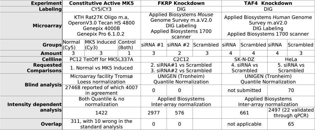
The second experiment involves the TATA binding protein Associated Factor 4 (TAF4). The transcription factor TFIID is a multiprotein complex composed of the TATA box-binding protein (TBP) and multiple TBP-associated factors (TAFs). TFIID plays an essential role in mediating transcriptional activation by gene-specific activators. TAFs have been postulated to exert several important roles in transcription acting as core promotor specificity factors and co-activators. Genetic studies in vertebrate cells also point to an essential role of TAFs in cell cycle progression [19, 20, 21, 22]. Using siRNAs we measured the influence of TAF4 depletion on the transcriptome (SiRNA will bind to the transcript and activate the destruction or prevent translation of the target sequence [23]). These experiments were performed in HeLa cells and SK-N-DZ cells. For each cell type we used 4 slides with scrambled siRNAs and 4 slides with TAF4-directed siRNA. The microarrays relied on DIG (digoxigenin) labeling.
The third experiment focuses on a putative glycosyltransferase. A number of congenital muscular dystrophies (CMD) are now known to be associated with mutations in genes encoding for proteins that are either putative or determined glycosyltransferases lending support to the idea that aberrant post-translational modifications of proteins may represent a new mechanism of pathogenesis in the muscular dystrophies. One of these genes, fukutin-related protein (FKRP), is thought to be coding for a putative glycosyltransferase, but its function has not yet been established [24]. To evaluate the possible effect of FKRP on transcription we transfected C2C12 cells with siRNA that targets FKRP. The results of the transfection were measured using microarray analysis using DIG labeling. Table 1 gives an overview of the different experiments.
2 Analysis Method
The presented analysis method measures the variance of a control sample, then uses it to model an intensity dependent error distribution and based on that defines confidence intervals for each individual spot, or group of spots. Regulations are reported as terms within a confidence interval of 95%. Conversion to ratios can be performed as necessary.
2.1 Acquiring the Error Model
To acquire the error model, one can employ two techniques. The first supplies a number of identical pairs of biological samples and puts them on different slides. For instance, one slide can contain the TAF4 downregulated transcript, while another slide contains the normal transcript. One can then use the inter-slide variance to develop an error model. A second approach, and the one used for the MK5 experiment, acquires the error on the regulation difference. In this setup, one provides the same sample for red and green. Because red and green have the same content one expects both channels to be equal for all spots. In the discussion below we assume that red and green name two samples that ought to be compared. Whether they are using Cy5/Cy3 staining or DIG labeling is irrelevant for the discussion.
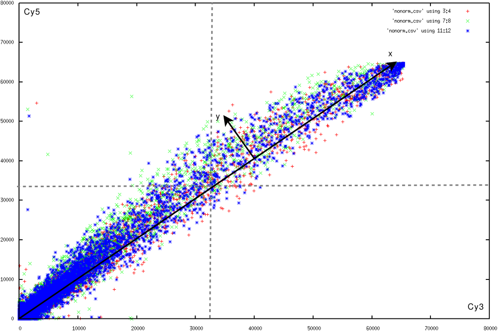
Figure 1 plots the red and green channel of such a control slide. We find that the variance around the expected values increases together with the spot intensity. This phenomenon indicates relative errors, and is the main reason why one relies on a log-transform. However, in the second half (with red or green intensities larger than 32768) the variance decreases with increasing spots intensity. A partial reason for this might lie in the number of saturated pixels.
 |
The above observation on the error distribution prohibits us to use
a maximum likelihood estimation of the absolute and relative errors
[16, 25].
Instead, we model a collection of
error distributions: one for each intensity. A two-dimensional map
will count the number of spots with a specific intensity and deviation.
Spot intensity (set out horizontally) is calculated as the mean of
the red and green channel. Spot deviation (set out vertically) is
red subtracted from green. Afterward, the algorithm normalizes the
two-dimensional histogram so that each intensity has: a) a proper
cumulative probability distribution and b) relies on enough samples
to have a good estimate of the modeled error. This process is detailed
in section 7 and results in two
functions
![]() and
and ![]() . They produce respectively a probability distribution
and cumulative probability distribution for each intensity (
. They produce respectively a probability distribution
and cumulative probability distribution for each intensity (![]() ).
).
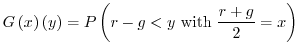
For illustrative purposes, we added ![]() and
and ![]() labels to Figure
1. Figure 2
plots the error distribution
of the MK5 experiment. When the error model is obtained from different
slides then the probability distribution
labels to Figure
1. Figure 2
plots the error distribution
of the MK5 experiment. When the error model is obtained from different
slides then the probability distribution ![]() (and associated cumulative
distribution
(and associated cumulative
distribution ![]() ) is based on the error model of each slide and convolved
accordingly.
) is based on the error model of each slide and convolved
accordingly.
|
2.2 Confidence Intervals on One Measurement
Assuming that the probability distribution ![]() expresses the error
distribution of a specific spot, and that
expresses the error
distribution of a specific spot, and that ![]() is the real (but unknown)
regulation, then our measurement
is the real (but unknown)
regulation, then our measurement ![]() will report a value in the range
will report a value in the range
![]() , in which
, in which ![]() satisfies
satisfies ![]() . In other
words, instead of measuring the real regulation, we will always measure
the real regulation with some extra unknown error. Since we know
. In other
words, instead of measuring the real regulation, we will always measure
the real regulation with some extra unknown error. Since we know ![]() and have some understanding of
and have some understanding of ![]() (its distribution) we can
state that
(its distribution) we can
state that ![]() . Thus, by determining a confidence interval
on
. Thus, by determining a confidence interval
on ![]() we can report
a confidence interval on
we can report
a confidence interval on ![]() as
well.
as
well.
A ![]() confidence
interval for spots with intensity
confidence
interval for spots with intensity ![]() is given
as
is given
as ![]() .
If a spot measures as
.
If a spot measures as ![]() , then in
, then in ![]() of the cases,
the real
regulation falls within
of the cases,
the real
regulation falls within
2.3 Reporting Regulations
A widely accepted method for quantitative measurement are log-ratios.
Despite widely used, they have a number of important limitations.
First, the log ratio cannot capture information such as the measurement
error. For instance the ratio 2/1 has probably more errors involved
than 2000/1000. The log![]() ratio will report 0.3 regardless.
Secondly, the log ratio has numerical problems near zero. An up- or
downregulation from zero to 1416 might make biological sense but it
seems inappropriate to express it as a (log-)ratio of
ratio will report 0.3 regardless.
Secondly, the log ratio has numerical problems near zero. An up- or
downregulation from zero to 1416 might make biological sense but it
seems inappropriate to express it as a (log-)ratio of ![]() .
.
To approach these challenges, our method reports the measured
regulation
as the difference between two slides, thereby including the lowest
and highest expected differences (Table 2).
In many cases this leads to an up- or
downregulation. Such
non-sensical regulations ought to be filtered out since the possible
error outweighs the actual measurement. Eg, a confidence interval
of ![]() for a spot with a
regulation of
for a spot with a
regulation of ![]() indicates that the real regulation-difference will range within
indicates that the real regulation-difference will range within ![]() .
Figure 3A illustrates a set of points omitted
due to
such filtering.
.
Figure 3A illustrates a set of points omitted
due to
such filtering.
When a consensus on the regulation exists (lowest boundary and highest
boundary have the same sign), we can calculate the regulation ratios
by assuming that either red or green could have been fully responsible
for the measurement error. In such extreme cases the highest ratio
can have a value of ![]() .
.
2.4 Confidence Intervals on Multiple Measurements
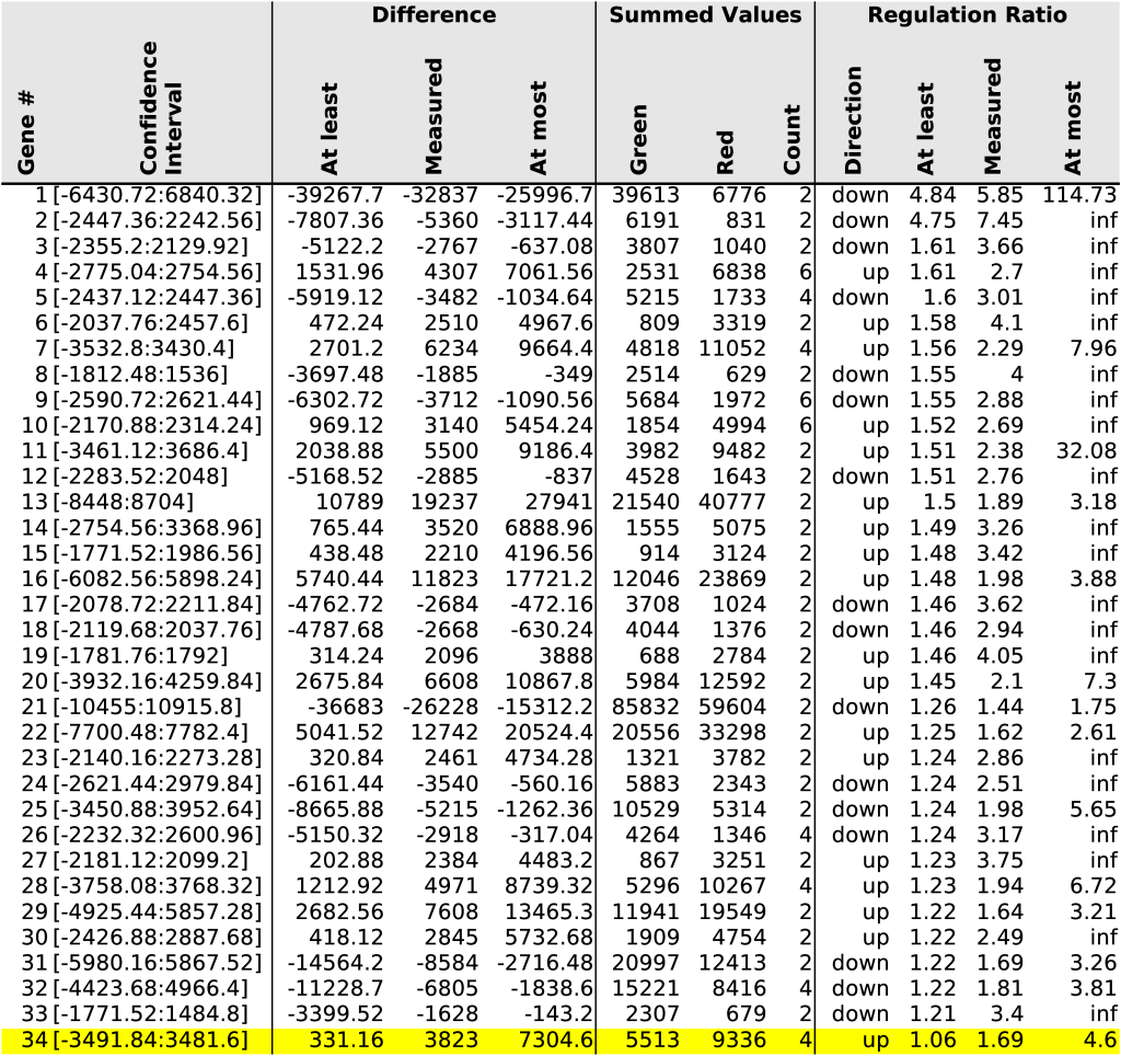
When multiple measurements are available, we can make the final confidence intervals smaller by convolving their respective probability functions. Section 7.4 covers the details. Table 2 illustrates the combination of oligosequences belonging to the same gene and consequently reports smaller confidence intervals.
As an illustrative example of the advantage of combining the
different
probability distributions we investigate gene #34 (Table 2).
The microarray measures this gene using two distinct probes, labeled
Rn30006190 and Rn30021393. On slide 1, Rn30006190 has an upregulation
in the range ![]() (measured as 999). On slide
2, it has an upregulation in the range
(measured as 999). On slide
2, it has an upregulation in the range ![]() (measured
as
(measured
as ![]() ). On slide 1, Rn30021393 has an upregulation in the range
). On slide 1, Rn30021393 has an upregulation in the range
![]() (measured as
(measured as ![]() ). On slide 2, it has
an upregulation in the range
). On slide 2, it has
an upregulation in the range ![]() (measured
as
(measured
as ![]() ). None of these individual measurements can tell us something
about the gene regulation since they all could have been downregulated
as well. However, by combining their error distributions we are able
to report that the overall gene is upregulated with at least a 6%
increase and at most a 4.6 times increase (last row of Table 2).
). None of these individual measurements can tell us something
about the gene regulation since they all could have been downregulated
as well. However, by combining their error distributions we are able
to report that the overall gene is upregulated with at least a 6%
increase and at most a 4.6 times increase (last row of Table 2).
3 Validation
We validated our method by means of qPCR and by comparing it to standard analysis protocols. For MK5 this analysis was performed at the Microarray facility in Tromsø. For the FKRP and TAF4 experiments, this analysis was performed by UNIGEN (Trondheim).
3.1 Quantitative PCR
To validate the regulations we found in the TAF4 experiment, we selected 22 genes and monitored their transcript levels by quantitative PCR (qPCR). Such qPCR results should be treated with caution. First, it is an inherent different measurement technique and thus it is unexpected that the results will completely fall within the reported confidence intervals. Secondly, the quantitative PCR experiment is often based on a new batch of cells, which means that the transfection efficiency can be different, and thus the actual results as produced in the qPCR can be a ratio higher or lower. A new batch was used for the TAF4 HeLa cells. The SK-N-DZ cells were based on the same batch. To account for the transfection efficiency, we performed a least square fit of the qPCR results to the microarray results. Thirdly, the primer sequences can be slightly different leading to different measurement efficiencies. Fourth, the housekeeping gene used in the qPCR experiment can be indirectly linked with the genes we measure, leading to a gene specific bias. And as a last remark, since we do not have an error model of the qPCR measurements, the dynamic range of the housekeeping gene might put a limitation on the qPCR accuracy. Notwithstanding these considerations, we performed 22 qPCR experiments, which confirmed that our technique is a valuable analysis method. Table 3 summarizes the results.
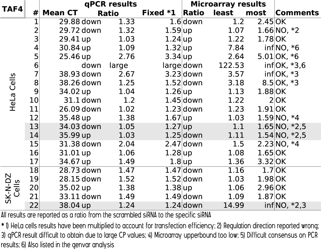 |
From the 22 measurements, 3 were not used because we could doubt both the PCR and microarray results. In particular, a number of qPCR measurements could be considered up or downregulated depending on the analysis process followed (eg. mean of ratios versus ratio of means). From the 19 remaining genes, 12 were fully correct, that is, the qPCR results fell within the reported confidence interval. For 2 genes, the predicted upperbound was too low. For 3 genes, the microarray reported strong regulations, however the qPCR measurement was unable to measure the exact value because the CP values were too large. For these genes it is very likely that the microarray reported correct. One gene did not match between both experiments. And for 1 gene the microarray experiments reported a confidence interval that was substantially larger than the qPCR value.
In the strictest sense (upperbounds and lowerbounds match), our method was able to match 79% of the qPCR results. If one is satisfied with proper lower bounds, then 89% of the results were reported accurately.
3.2 FKRP and TAF4
Next to the qPCR validation, we compared our method to a blind analysis by other groups. The blind analysis for the FKRP and TAF4 experiments followed the guidelines of [26]. The PCA analysis revealed no outlier for any of the slides. The analysts attempted to gage the genetic variations (abbreviated: genvar) between the different slides and then report those that changed significantly. For the TAF4 HeLa cells experiment, the genvar error model reduced the dataset to 70 significant genes, while the intensity dependent analysis (abbreviated: indep) retained 2497 genes (The TAF4 SK-N-DZ was not sent for analysis, but to be complete, we found 661 to be significant). Five genes were only reported in the genvar set. Those 5 were all below the average gene intensity and the mismatch may be due to the normalization differences (quantile vs Applied Biosystems) or microarray outliers. We would liked to have validated those 5 mismatches through qPCR, but no probe sequences, nor gene annotations were available, so we could not verify them. The previous 22 qPCR measurements did however include 3 genes that were reported in the genvar analysis. Two of these produced qPCR values with large CP values (thus with a high error rate), thereby offering little extra information. For the FKRP experiment there were no significant alterations which was, according to the report, due to the few samples we provided (4 replicas vs 3 replicas). The indep analysis reported 2977 regulations for the siRNA#1 group and 576 regulations for the siRNA#2 group.
Compared to a standard analysis, our method reported more genes. In the TAF4 experiment, we found 35x more genes than the standard analysis. Most of these genes could be validated with qPCR, leading to the conclusion that standard analysis methods may be too stringent.
3.3 MK5
The standard microarray analysis, based on loess normalization [1, 2], contained 27648 spots for each slide, of which 4007 pairs in agreement (both slides reporting the same qualitative regulation, being up or down). Based on both slides, our method only reported 1422 spots. Three hundred and eleven spots occurred in both methods, 1111 spots were unique to our analysis and 3696 spots were unique to the standard analysis.
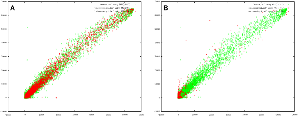 |
To better understand the differences in reported genes, it is helpful to include a picture (Figure 3) that illustrates both the variance on the measurements and the samples we removed/retained.
The first consideration regards spots that occurs in the loess set but not in our analysis. Is there a good reason why we should not take those particular data points into account ? Figure 3A illustrates the spots that only occurred in the loess set (red) as well as the variance of the experiment (green). Clearly, the omitted spots were too close within the expected variance to be useful.
The second concern regards those spots that only occurred in our analysis. These are pictured in Figure 3B. The main reason why our method was more sensitive and could report them lies in the convolution of the error distributions of similar spots. This information was unavailable to the loess method since there we were forced to stick to a more rigid approach that both slides agreed qualitatively.
The last concern regards overlapping spots. All of them should
report
at least the same qualitative regulation. From the 311 spots, 10 failed
to do so. Looking at the non-normalized data (Table 4)
we find that all spots were correctly reported by the confidence
interval
method. The reason why the loess method failed, probably lies in the
model fitting that will inevitable position certain spots at the wrong
side of the zero-line (a ratio of 2 is after all closely located to
zero when expressed as a log![]() ratio).
ratio).
 |
4 Discussion
Our method was validated using qPCR and we found that it reports useful confidence intervals (79% correct, 89% when omitting the upper limit). We also found that the method surpasses standard methods in the number of genes it reports (x35 in our case).
4.1 Difference between machines, cell lines and experiments
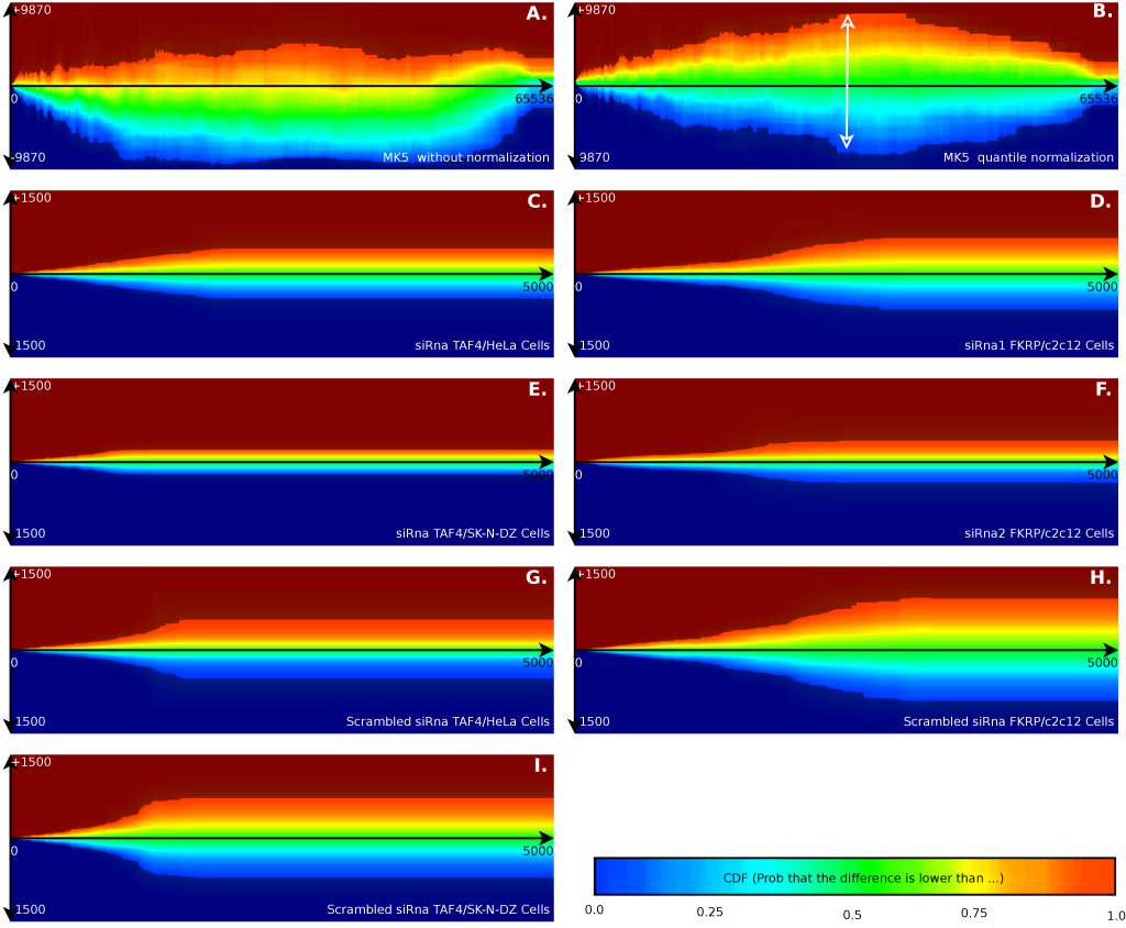
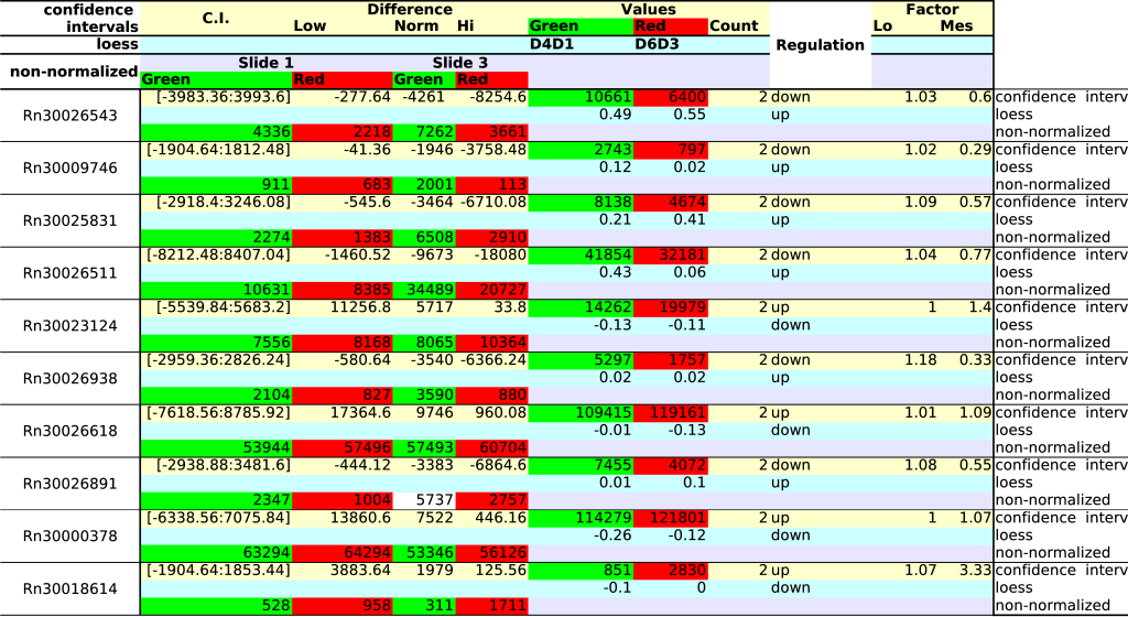
The sampling of the error distribution is specific to the gain of the acquisition hardware, the biological sample, the slide quality, slide facturer, supplier of the microarray hardware, temperature, sample handling and probably many more influences. Therefore, the error model must be developed for each specific experiment. This is illustrated in Figure 2, which visualizes the difference between a number of these variables.
- We illustrated the technique on a knockdown of a gene as well as on a constitutive active gene. Figures 2A & B are the constitutive active MK5. Figures 2C, D, E & F are those with a knockdown of a gene. These figures also illustrate the technique on two different scanners. Figures 2A & B are made on a Tecan scanner with Cy5/Cy3 labeling. All others are made with DIG labeled slides scanned on an Applied Biosystems 1700 scanner.
- Figures 2G, H & I versus Figures 2C, D, E & F illustrate the differences between scrambled siRNA and specific siRNA. The results show that scrambled siRNA introduces more variability in the cell system than previously anticipated. This might suggest that a scrambled siRNA alone as a negative control might not be sufficient, or will in a sense, reduce the number of useful results that can be obtained from this type of experiment.
- We illustrated the technique on the same experiment, but with different cell types. Figures 2C, G are performed in HeLa cells, while Figure 2E, I plots the data from SK-N-DZ cells. Compared to the FKRP experiments, they reach their maximum variability point at lower intensities. Between the two different cell types we find that the SK-N-DZ cells reached their maximum variability point also at lower intensities.
- Figure 2D plots siRNA#1 while Figure 2F plots the siRNA#2, which target slightly different FKRP mRNA. The small variations in Figure 2F might suggest that we would obtain more data from this experiment. This however is incorrect. For siRNA#2 we only obtained 576 valuable genes, while the siRNA#1 group produced 2977 genes. This probably happened due to either a bad transfection efficiency (leading to low variations, but also to little useful data) or a low siRNA#2 impact in general. This illustrates that the size of the error as such does not provide much information, it must always be related to the impact of the cell alteration itself.
- Figures 2D, F, H are mouse survey gene arrays, while Figures 2C, E, G, I are human genome survey arrays. We find little overall impact of the type of array in the shape of the error plots.
- Figure 2A is made using Cy5/Cy3 labeling without normalization. Figure 2B is the same figure but relying on quantile normalization. Figure 2C-I are based on the applied biosystem inter array normalization algorithm. The differences in confidence intervals between Figure 2A and Figure 2B illustrates how our algorithm can model the inter-filter effect [10]. Instead of having a flat 'eye-shaped' error model (Figure 2B), one finds back a banana-shaped error model. This means that the model is independent from a particular normalization to account for light reabsorption. Using confidence intervals, there is no particular need to perform separate dye specific normalizations.
4.2 Optimal areas of measurement
Looking at the results (Figure 2 and 3B), our observations do not support the general believe that 'bright spots are good spots'. Actually, we find that intense spots are subject too much larger errors. Therefore we might wonder whether there are measurement areas that produce the most information. In our MK5 error model we find that the bright spots are the ones that should be removed from the data set since they are too close to the expected error, while the darker spots often fall outside the measurement error (see Figure 3A). Figure 3B illustrates this further: contrary to what one would expect we find the largest collection of useful spots at the edges around the origin.
4.3 Amplification errors seem to outweigh genetic variability
Given the considerations these days on genetic pathways and genetic variability, we now discuss how these two factors influence our analysis method. The first concern is that certain genes have a larger natural variability (unstable expressed genes) than other, more stably expressed, genes. Since our method does not assess genetic variability, it might omit significant changes in stable expressed genes if they are too close to each other. It might also report highly unstable expressed genes as significantly altered while, in reality, they might just have fallen outside the confidence interval by chance. While there may be such genes, our initial observations does not seem to be influenced by it. Our PCR results confirm our confidence intervals, which seems to indicate that the impact of genetic variability is much lower than anticipated. Instead we find that the experimental variability, cell perturbation and consequent amplification/propagation cascades outweighs natural genetic variability.
The second concern addresses genetic pathways: the gene expression pattern in a cell is the result of a cascade event, where products of primary gene transcripts can affect the expression of other genes. Of course, when measuring the same samples, one still expects to find the same values (eg. in Figure 1, regardless of the gene linking, the control should be a straight line). However, if an error or a variability occurs in the initial perturbation, then it is not unexpected that this error will propagate along the same pathways. This effectively leads to a cascade of expression patterns, in which every step can reduce or increase the net output effect. In other words, the amount of transcribed gene can be dependent on the amount of transcripts of linked genes, but multiplied with an unknown factor. Very seldom will we find that one expression pattern produces a new expression pattern with exactly the same amount of transcripts. So, by pooling together a random set of transcripts based on their intensity, we substantially limit the impact of genetic pathways. In the worst case scenario, if there were a significant collection of dependent transcripts, all with the same expression levels, then they would be placed in the same intensity-slice, thereby sharpening the probability distribution on that slice. This would in turn lead to a list of genes that could contain non-significantly altered gene expressions. In our work, we did not find much evidence that our intensity-based pooling is inadequate and/or overly sensitive to genetic pathways. The entire collection of probability distributions was in all our experiments smooth without outliers.
4.4 Lorentz distributions
We believe that the presented method makes a fair trade off between a full understanding the gene linkages/variations (which is something we cannot measure with 3 or 4 slides) and error models that do not take such possibility into account at all. Standard microarray error models are often based on the log-scale of the two channels (red/green or slide1/slide2) [27, 15]. The resulting distributions appear as a Lorentz distribution [15, 16]. However, such distributions cannot capture relative errors in the experimental process. This leads to standard error models that are too wide for low intensity spots and too small for high intensity spots.
4.5 Gating
Aside from the advantages listed above we also found an interesting side observations, which was a form of gating on the Tecan scanner. Figure 4 plots the one dimensional distribution of all intensities, and one would expect either a Lorentz distribution [16] or a normal distribution, instead we find something in between that has a plateau around zero (marked with a red circle).
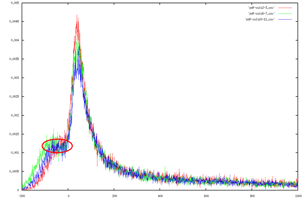 |
We marked the plateau with a red circle (See Figure). At this point, we have merely been speculating about an explanation for this local uniformity
- The plateau is not related to an error in the background subtraction because that would widen the entire probability distribution.
- A hybridization problem might have occurred. This will place many dots around 0. This however is not consistent with the scatterplot, which does not hint at such a large non-hybridization rate. Since all microarrays had a similar distribution, this becomes very unlikely.
- The microarray age might be an explanation, but this should not have occurred since we bought them just before the experiment.
- The electronics of the microarray scanner might be subject to a form of gating [12]. This will produce random results for a signal until the signal is strong enough to be picked up properly. Because we did not see the same plateau at low intensities, this might hold some ground.
- Highly speculative is a chemical critical mass of sorts that will randomly fluctuate unless there is enough material to produce a stronger signal.
- A systematic production error on the microarray slides, but this is difficult to verify without close cooperation with the slide fabricator.
- It might be a specific feature of the MK5 cell system, with a large collection of genes only marginally expressed.
4.5.0.1 Deconvolution of error distributions
Regarding future work, we might improve the method through deconvolution of the DIG labeled error distributions. When acquiring the error model based on the differences between replica slides, one actually measures the auto-convolved error distribution. As such, it will be slightly larger than the real error distribution. This can be improved through deconvolution techniques such as adaptations to the Richardson-Lucy algorithm [28], but in general seems unnecessary.
5 Conclusion
We presented a method to analyze differences between groups of microarrays, such as often found in differential gene expression experiments. Instead of reporting one single number for each regulation, we report the regulation including its confidence interval. The confidence interval is obtained from an error model that must be measured within the experiment itself.
We compared our method to a standard analysis method and illustrated its capability to filter out spots that are too close to the error to be useful. For indicative purposes we compared the reported results to standard analysis methods. We also performed a limited qPCR experiment. Although a relative small number of samples have been investigated, they support the credibility of our analysis method.
6 Material and Methods
Manufacturers instruction are used unless stated otherwise.
6.1 Constitutive active MK5 cell-line
To clone the cDNA sequence of MK5, we introduced two mutations in
the pcDNA-HA-MK5![]() plasmid [29]. Both used the
Stratagene mutagenesis kit. The first mutation assured compatibility
with the pTRE2 plasmid and used a forward primer
5'-CCC-AAG-CTT-GAC-GCG-TCC-ATG-TAT-GAT-G-3'
with complementary reversed primer. The second mutation turned the
wt MK5 into a constitutive active MK5
plasmid [29]. Both used the
Stratagene mutagenesis kit. The first mutation assured compatibility
with the pTRE2 plasmid and used a forward primer
5'-CCC-AAG-CTT-GAC-GCG-TCC-ATG-TAT-GAT-G-3'
with complementary reversed primer. The second mutation turned the
wt MK5 into a constitutive active MK5![]() mutant. The resulting
MK5 cDNA sequences were excised by MluI/NotI digestion
and cloned into the corresponding sites of pTRE2. We verified the
plasmid by sequencing. Two 6-well plates with
mutant. The resulting
MK5 cDNA sequences were excised by MluI/NotI digestion
and cloned into the corresponding sites of pTRE2. We verified the
plasmid by sequencing. Two 6-well plates with ![]() PC12 TetOff
cells (BD Biosciences) were transfected with 14
PC12 TetOff
cells (BD Biosciences) were transfected with 14![]() g of pTRE2-MK5
g of pTRE2-MK5![]() and 2
and 2![]() g pTKHyg per well using lipofectamine 2000 (Invitrogen)
[30]. After
g pTKHyg per well using lipofectamine 2000 (Invitrogen)
[30]. After ![]() h, the medium was changed
and supplemented with
h, the medium was changed
and supplemented with ![]() ng/ml Doxycycline (Sigma).
ng/ml Doxycycline (Sigma). ![]() h after
transfection, cells were transferred to 10 cm dishes with fresh medium
and Doxycycline.
h after
transfection, cells were transferred to 10 cm dishes with fresh medium
and Doxycycline. ![]() h after transfection, 100
h after transfection, 100![]() g/ml of Geneticin
(Gibco) and 200
g/ml of Geneticin
(Gibco) and 200![]() g/ml Hygromycin B (Invitrogen) was supplied
additionally to the medium. The cells were grown until visible colonies
of resistant cells could be detected. From each plate two colonies
were transferred in threefold dilution to a
g/ml Hygromycin B (Invitrogen) was supplied
additionally to the medium. The cells were grown until visible colonies
of resistant cells could be detected. From each plate two colonies
were transferred in threefold dilution to a ![]() well plate. For
positive clones, we confirmed the transgene expression though reverse
transcriptase-PCR and western blot. Cells were maintained in DMEM
supplied with
well plate. For
positive clones, we confirmed the transgene expression though reverse
transcriptase-PCR and western blot. Cells were maintained in DMEM
supplied with ![]() horse serum
and
horse serum
and ![]() fetal bovine serum, 2mM
L-glutamine, penicillin (110 units/ml) and streptomycin (100
fetal bovine serum, 2mM
L-glutamine, penicillin (110 units/ml) and streptomycin (100![]() g/ml).
Additionally, 50
g/ml).
Additionally, 50![]() g/ml of Geneticin, 100
g/ml of Geneticin, 100![]() g/ml Hygromycin B
were supplied to maintain selection. To suppress HA-MK5
g/ml Hygromycin B
were supplied to maintain selection. To suppress HA-MK5![]() expression during ordinary cell culture, we added 10ng/ml Doxycycline.
expression during ordinary cell culture, we added 10ng/ml Doxycycline.
6.2 TAF4/FKRP knock-down using siRNAs
SiRNAs introduced into the cells lead to degradation of mRNA having
the complementary sequence, thereby silencing/depressing gene
expression.
SiRNAs were pre-designed and ordered from Qiagen
(http://www.qiagen.com/).
For the FKRP experiment, the siRNAs sequences targeted
AACCTCCTAGTCTTCTTCTAT;
AACCCAAAGACTGGAGCAACT. For the TAF4 experiments, the siRNA targeted
AAGGCCTGTGGATACTCTTAA . Cells were plated at ![]() cells/ml into
a 6-well dish. Because of different growth-rates, HeLa and C2C12 cells
were transfected after
cells/ml into
a 6-well dish. Because of different growth-rates, HeLa and C2C12 cells
were transfected after ![]() hours, while SK-N-DZ cells were transfected
after more than
hours, while SK-N-DZ cells were transfected
after more than ![]() hours. Two
different transfection mixes were
made. Both included 90 vol% D-MEM(SBS). The first transfection mix
contained 10 vol% TAF4 siRNA (30nM siRNA/well). The second transfection
mix contained 10 vol% scrambled siRNA. The different mixes were
vortexed,
hours. Two
different transfection mixes were
made. Both included 90 vol% D-MEM(SBS). The first transfection mix
contained 10 vol% TAF4 siRNA (30nM siRNA/well). The second transfection
mix contained 10 vol% scrambled siRNA. The different mixes were
vortexed,
![]()
![]() l RNAiFect was added and then incubated for 15
minutes (room temperature). D-MEM was aspirated from the wells.
Subsequently,
l RNAiFect was added and then incubated for 15
minutes (room temperature). D-MEM was aspirated from the wells.
Subsequently,
![]()
![]() l of the transfection mixture was added to each
well in addition to
l of the transfection mixture was added to each
well in addition to ![]() ml fresh D-MEM (10% FBS + antibiotics).
We produced each transfection mix in triplicate. Twenty-four hours
after transfection, RNA was to be extracted for further analysis.
The same procedure was followed in the FKRP knockdown experiments.
ml fresh D-MEM (10% FBS + antibiotics).
We produced each transfection mix in triplicate. Twenty-four hours
after transfection, RNA was to be extracted for further analysis.
The same procedure was followed in the FKRP knockdown experiments.
6.3 RNA extraction and cDNA Synthesis
C2C12 (FKRP), HeLa (TAF4) and SK-N-DZ (TAF4) cells were plated at
![]() cells per well in a
cells per well in a ![]() well dish; MK5 stable cells at
well dish; MK5 stable cells at
![]() cells per 6 well dish. For
the TAF4 and FKRP experiment,
cells were lysed by incubation in lysis buffer containing chaotropic
salt and Proteinase K, after which RNA was isolated with the MagNA
Pure Compact RNA system (Roche-Applied-Science). For the MK5
experiment,
we used the Nucleospin II RNA isolation kit (Machery-Nigel). The
Nanodrop
ND-1000 (Nanodrop technologies Inc.) verified RNA concentrations and
purity. One
cells per 6 well dish. For
the TAF4 and FKRP experiment,
cells were lysed by incubation in lysis buffer containing chaotropic
salt and Proteinase K, after which RNA was isolated with the MagNA
Pure Compact RNA system (Roche-Applied-Science). For the MK5
experiment,
we used the Nucleospin II RNA isolation kit (Machery-Nigel). The
Nanodrop
ND-1000 (Nanodrop technologies Inc.) verified RNA concentrations and
purity. One ![]() g of RNA was reverse transcribed to cDNA using the
iScript cDNA synthesis kit (Biorad) (MK5) and SuperScript
g of RNA was reverse transcribed to cDNA using the
iScript cDNA synthesis kit (Biorad) (MK5) and SuperScript![]() II
from Invitrogen
II
from Invitrogen![]() (remaining
experiments).
(remaining
experiments).
6.4 Quantitative Realtime PCR TAF4 related genes
We made 4 cDNA dilutions: 1:2, 1:5, 1:10 and 1:50. All were
supplemented
with mastermix, primers, probe and water. Relative expression for
each target gene was normalized to GAPDH using the 2
![]() method [31]. The expression differences
between scrambled
and normal siRNA were calculated by dividing the averages of each
cell type. The qPCR experiments were performed on LightCycler 480
(Roche), with accompanying software version 1.2.0.0625.
method [31]. The expression differences
between scrambled
and normal siRNA were calculated by dividing the averages of each
cell type. The qPCR experiments were performed on LightCycler 480
(Roche), with accompanying software version 1.2.0.0625.
6.5 Microarray
The number of slides and their layout is provided in Table 1. For the MK5 experiment, we made 3 slides, each containing an induced (Cy3) and uninduced sample (Cy5). The 4th slide contained two induced samples. Samples were labeled with the 3DNA 350S HS labeling kit (Genisphere). Hybridized slides were scanned using the Genepix 4000B (Molecular Devices) with a constant gain of 950/800. We obtained more than 70% hybridization (measured as #spots > median + 1SD). Spots with too large an intensity (> 90% of the maximum) or too large a regulation (> x10) were removed. For standard analysis, we relied upon a blind analysis of the microarray facility in Tromsø, which used loess normalization [1]. Our own analysis used quantile normalization [3]. For the FKRP & TAF4 experiments, we used an Applied Biosystems 1700 scanner, with AB. v2.0 slides surveying respectively the mouse genome and human genome. UNIGEN in Trondheim performed a blind data analysis following the guidelines of [26]. This included quantile normalization on the raw machine output. Our analysis was based on the already normalized output of the Applied Biosystems scanner.
7 Detailed Analysis Method
7.1 Notation
We denote every slide with a number which is placed top-right. The
control slide is marked with a ![]() . In the bottom-right we refer
to either the red or green channel. Eg
. In the bottom-right we refer
to either the red or green channel. Eg ![]() refers to the
red channel of spot
refers to the
red channel of spot ![]() in slide
in slide ![]() . Each channel must be measured,
with or without quantile normalization, but always without taking
the logarithm. The maximum measurable value is expressed as
. Each channel must be measured,
with or without quantile normalization, but always without taking
the logarithm. The maximum measurable value is expressed as ![]() ,
which typically is
,
which typically is ![]() (this is the maximum value that can be
expressed using
(this is the maximum value that can be
expressed using ![]() bits). The
dataset is preferably already filtered
for false positives. The norm of a spot
bits). The
dataset is preferably already filtered
for false positives. The norm of a spot ![]() is written as
is written as
The difference between the two channels is subscribed with a ![]() subscript. Eg
subscript. Eg ![]() .
.
7.2 Creating Histograms
We model the error distributions as a collection of histograms in
function of spot intensity. We rely upon ![]() bins, each in which
we store a histogram. We denote
bins, each in which
we store a histogram. We denote ![]() the histogram for bin
the histogram for bin ![]() .
It will cover all the spots within intensity range
.
It will cover all the spots within intensity range ![]() .
The histogram
.
The histogram ![]() counts the
occurrences of a specific intensity.
Using
counts the
occurrences of a specific intensity.
Using ![]() bins,
bins, ![]() will cover all the spots for
which
the difference lies within
will cover all the spots for
which
the difference lies within ![]() .
The creation of these histograms obviously starts with each
.
The creation of these histograms obviously starts with each ![]() .
The algorithm below calculates the 2 dimensional histogram.
.
The algorithm below calculates the 2 dimensional histogram.
-
- foreach spot


7.3 Smoothing
After performing this process we smoothen out the distribution along
the intensity axis. This ensures that each histogram contains a minimum
amount of measurement-error measurements. The smoothing is performed
adaptively by widening a window around each intensity until enough
points are gathered. If we call ![]() the minimum mass of each
histogram, then the algorithm below will create a smoothed collection
of probability distributions and store it in
the minimum mass of each
histogram, then the algorithm below will create a smoothed collection
of probability distributions and store it in ![]() .
.
-
- foreach intensity


do

while

7.4 Multiple
Measurements
Assume that we have a set of spots ![]() , all measuring the same process
(eg the same oligosequence, or the same gene), then we can define
the overall measurement
, all measuring the same process
(eg the same oligosequence, or the same gene), then we can define
the overall measurement ![]() as
as
![]() and
and ![]() .
Then we also have that
.
Then we also have that

The error distribution associated with a specific spot is written
as ![]()
For each value of ![]() we have an associated error
distribution.
The overall error distribution for
we have an associated error
distribution.
The overall error distribution for ![]() will consequently
be the convolution of the underlying error distributions (written
as
will consequently
be the convolution of the underlying error distributions (written
as ![]() ).
).
7.5 Confidence Intervals
The confidence interval of ![]() associated with
associated with ![]() , given the
error distribution
, given the
error distribution ![]() is given by
is given by
![$\displaystyle \left[\mbox{CDF}_{\widetilde{m}}^{-1}\left(\frac{1-\kappa}{2}\right),\mbox{CDF}_{\widetilde{m}}^{-1}\left(\frac{\kappa+1}{2}\right)\right]$](img103.png)
![]() and
and ![]() are the lowest and highest boundaries for
measurement
are the lowest and highest boundaries for
measurement
![]() .
.
7.6 Regulation Factors
Converting absolute regulation differences to regulation ratios
requires
that we assume that either ![]() or
or ![]() could have
been fully
responsible for the measurement error. This leads to the following
possible regulation ratios:
could have
been fully
responsible for the measurement error. This leads to the following
possible regulation ratios:
Min![]() reports the lowest possible regulation ratio. Max
reports the lowest possible regulation ratio. Max![]() reports the highest possible regulation ratio.
reports the highest possible regulation ratio.
8 Acknowledgments
Lotte Olsen and Jørn Leirvik for performing the microarray experiment and Halvor Sehested Grønaas for conducting the loess normalization on the MK5 data. All three worked at LabForum at that time. Endre Anderssen (UNIGEN/Trondheim) performed the blind analysis of the TAF4 and FKRP datasets. The Norwegian Research Council (grant 160999/V40) and the Norwegian Cancer Society (project A01037) supported the MK5 experiments. Helse Nord (project SFP-114-04) supported the TAF4 project. Helse Nord HF supported the FKRP project. The University of Tromsø (``Miljøstøtte'') and the University Hospital of Northern Norway equally supported this particular research.
9 Authors Contributions
Werner Van Belle invented and implemented the presented technique and wrote the manuscript. Nancy Gerits created the constitutive active MK5 cell line, designed and performed the MK5 experiments and helped writing the manuscript. Kirsti Jakobsen performed the TAF4 experiments, performed the qPCR experiments and provided substantial input in the manuscript. Vigdis Brox performed the FKRP experiments. Marijke Van Ghelue designed the TAF4 and FKRP study and helped writing the manuscript. Ugo Moens designed the MK5 experiment, helped designing the TAF4 experiment and helped writing the manuscript.
Bibliography
| 1. | Statistical Models in S W. S. Cleveland, E. Grosse, W. M. Shyu Wadsworth \& Brooks/Cole; editor: J. M. Chambers and T. J. Hastie; chapter: Local Regression Models; 1992 |
| 2. | Normalization of cDNA Microarray Data G. K. Smyth, T. P. Speed Methods; volume: 31; pages: 265-273; 2003 |
| 3. | Statistical Methods for Identifying Differentially Expressed Genes in Replicated cDNA Microarray Experiments Sandrine Dudoit, Yee Hwa Yang, Matthew J. Callow, Terence P. Speed institution: Department of Biochemistry, Stanford University School, Beckman Center B400, Stanford CA 94305-5307; 2000 |
| 4. | A Neural Network-Based Similarity Index for Clustering DNA Microarray Data T. Sawa, L. Ohno-Machado Comput Biol Med; volume: 33; number: 1; pages: 1-15; Jan; 2003 |
| 5. | Singular Value Decomposition for Genomewide Expression Data Processing and Modeling O. Alter, P. O. Brown, D. Botstein Proc. Natl. Acad. Sci. USA; volume: 97; number: 18; pages: 10101-10106; 2000 |
| 6. | Accounting for Probe-Level Noise in Principal Component Analysis of Microarray Data Guido Sanguinetti, Marta Milo, Magnus Rattray, Neil D. Lawrence Bioinformatics; volume: 21; number: 19; pages: 3748-3754; 2005 |
| 7. | Extraction of Correlated Gene Clusteres by Multiple Graph Comparison A. Nakaya, S. Goto, M. Kanehisa Genome Inform.; volume: 12; pages: 44-53; 2001 |
| 8. | The Advantage of Functional Prediction based on Clustering of Yeat Genes and its Correlation with non-sequence based Classifications Y. Bilu, M. Linial J. Comput Biol.; volume: 9; number: 2; pages: 193-210; 2002 |
| 9. | Sources of nonlinearity in cDNA microarray expression measurements Latha Ramdas, Kevin R. Coombes, Keith Baggerly, Lynne Abruzzo, W. Edward Highsmith, Tammy Krogmann, Stanley R. Hamilton, Wei Zhang Genome Biol.; volume: 2; number: 11; 2001 |
| 10. | Experimental correction for the inner-filter effect in fluorescence spectra M. Kubista Analyst; volume: 119; pages: 417-419; 1994 |
| 11. | Stability, specificity and fluorescence brightness of multiply-labeled fluorescent DNA probes J.B. Randolph, A.S. Waggoner Nucleic Acid Res.; volume: 25; number: 14; pages: 2923-2929; Jul; 1997 |
| 12. | Optical technologies for the read out and quality control of DNA and protein microarrays Michael Schäferling, Stefan Nagl Analytical and Bioanalytical Chemistry; volume: 385; number: 3; pages: 500-517; June; 2006 |
| 13. | Saturation and Quantization Reduction in Microarray Experiments using Two Scans at Different Sensitivities Jorge García de la Nava, Sacha van Hijum, Oswaldo Trelles Statistical Applications in Genetics and Molecular Biology; volume: 3; number: 1; 2006 |
| 14. | Profound influence of microarray scanner characteristics on gene expression ratios: analysis and procedure for correction Heidi Lyng, Azadeh Badiee, Debbie H Svendsrud, Eivind Hovig, Ola Myklebost, Trond Stokke BMC Genomics; volume: 5; number: 10; 2004 |
| 15. | Significance and statistical errors in the analysis of DNA microarray data James P. Brody, Brian A. Williams, Barbara J. Wod, Stephen R. Quake Proceedings of the National Academy of Sciences; volume: 99; pages: 12975-12978; 16 September; 2002 |
| 16. | Numerical Recipes in C++, The art of Scientific Computing William H. Press, Saul A. Teukolsky, William T. Vetterling, Brian P. Flannery Cambridge University Press; chapter: 15.7 Robust Estimation; pages: 704-708; edition: 2nd; 2003 |
| 17. | MAPKAP kinases - MKs- two's company, three's a crowd Matthias Gaestel Nature Reviews Molecular Cell Biology; volume: 7; pages: 120-130; 2006 |
| 18. | Cyanine Dye Labeling reagents: sulfoindocyanine succinimidyl esters R.B. Mujumdar, L.A. Ernst, S.R. Mujumdar, C.J. Lewis, A.S. Waggoner Bioconjug Chem; volume: 4; number: 2; pages: 105-111; Mar-Apr; 1993 |
| 19. | Transcriptional coactivator complexes A.M. Naar, B.D. Lemon BD, R. Tjian Annu Rev Biochem; volume: 70; pages: 475-501; 2001 |
| 20. | New insights into TAFs as regulators of cell cycle and signaling pathways I. Davidson, D. Kobi, A. Fadloun, G. Mengus volume: 4; number: 11; pages: 1486-1490; Nov; 2005 |
| 21. | The general transcription machinery and general cofactors M.C. Thomas, C.M. Chiang Crit Rev Biochem Mol Biol; volume: 41; number: 3; pages: 105-78; May-Jun; 2006 |
| 22. | TAFs revisited: more data reveal new twists and confirm old ideas S.R. Albright, R. Tjian Gene; volume: 242; number: 1--2; pages: 1-13; Jan 25; 2000 |
| 23. | Functional Anatomy of siRNA for mediating efficient RNAi in Drosophila Melanogaster embryo lasate. S.M. Elbashir The Embryo Journale; volume: 20; number: 23; pages: 6877-6888; 2001 |
| 24. | The gene for a novel glycosyltransferase is mutated in congenital muscular dystrophy MDC1C and limb girdle muscular dystrophy 2I. M. Brockington, D.J. Blake, S.C. Brown, F.Muntoni Neuromuscul Disord; volume: 12; number: 3; pages: 233-234; Mar; 2002 |
| 25. | Testing for Differentially Expressed Genes by Maximum-Likelihood Analysis of Microarray Data T. Ideker, V. Thorsson, A.F.Siegel, L.E.Hood Journal of Computational Biology; volume: 7; pages: 805-818; 2000 |
| 26. | Microarray Data Analysis: frmo disarray to consoloditation and consensus D.B. Allison, X. Cui, G.P. Page, M. Sabripour Nature Reviews Genetics; volume: 7; number: 1; pages: 55-65; Jan; 2006 |
| 27. | Error models for microarray intensities Wolfgang Huber, Anja von Heydebreck, MAtrin Vingron Encyclopedia of Genomics, Proteomics and Bioinformatics; John Wiley \& Sons Ltd.; editor: Michael Dunn and Lynn Jorde and Peter Little and Shankar Subramaniam; March; 2004 |
| 28. | Application of the Richardson-Lucy algorithm to the deconvolution of two-fold probability density functions. Gilbert Ricort, Henri Lantéri, Eric Aristidi, Claude Aime Pure Applied Optics; volume: 2; pages: 125-143; 1993 |
| 29. | Both binding and activation of p38 MAPK play essential roles in regulation of nucleocytoplasmic distribution of MAPK activated protein kinase 5 by cellular stress Ole Morten Seternes, Bjarne Johansen, Beate Hegge, Mona Johannessen, Stephen M. Keyse, Ugo Moens Molecular and cellular biology; volume: 22; number: 20; pages: 6931-6945; 2002 |
| 30. | Up-regulation of c-Jun N-terminal kinase pathway in Friedreich's ataxia cells Luigi Pianese, Luca Busino, Irene De Biase, Tiziana de Cristofaro, Maria S. Lo Casale, Paola Giuliano, Antonella Monticelli, Mimmo Turano, Chiara Criscuolo, Alessandro Filla, Stelio Varrone, Sergio Cocozza Human Molecular Genetics; volume: 11; number: 23; pages: 2989-2996; 2002 |
| 31. | Analysis of relative gene expression data using real-time quantitative PCR and the 2(-Delta Delta C(T)) Method. D.J. Livak, T.D. Schmittgen Methods; volume: 25; number: 4; pages: 402-408; December; 2001 |
| http://werner.yellowcouch.org/ werner@yellowcouch.org |  |