| Home | Papers | Reports | Projects | Code Fragments | Dissertations | Presentations | Posters | Proposals | Lectures given | Course notes |
|
|
Classification of Rhythmical PatternsWerner Van Belle1 - werner@yellowcouch.org, werner.van.belle@gmail.com Abstract : We classify rhythmical patterns using a variety of classifiers and report on the results. In summary: they do not directly seem useful to help us classify tempo multiples properly. However, as a side effect of this research we found a hint that a flux based measurement (how fast energy changes in a song) might be a useful idea to classify music into slow or fast classes.
Keywords:
rhythm classification, flux based measurement, fast slow songs |
Table Of Contents
Introduction
In [1] we figured out that measuring the tempo within a range of 11.25 to 22.5 MPM (45 to 90 qMPM) would lead to accurate measurements in 95% of the cases. That high accuracy could only be attained if we allowed the algorithm to report a multiple of the tempo. That is to say, we counted the reported tempo correct if it was close to the actual tempo, but also when its double was close to the correct tempo. Although that result seems somewhat lacking in rigor, it still remains an important result because we reduced a multi-class classification problem (there are many more tempo-multiples than *1 or *2), to a binary classification problem.
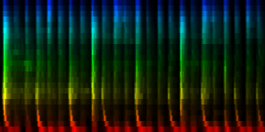
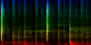
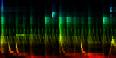
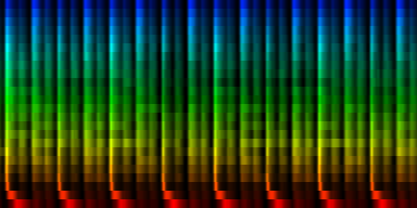
We believe that the rhythmical structure of music holds the key to recognizing the proper multiple. For instance in the image below, we see two rhythm patterns. The right one contains 8 beats per measure, which leads us to a conclusion that it might actually be two measures instead of one, so doubling the tempo will bring such measure back to 4 beats.
Consequently, we started to extract rhythmical patterns in such a manner that we would remove a number of confounding factors, such as sound color, echoes, rotational offsets etc [2]. The next step is now to use these extracted rhythms to obtain help in deciding the proper multiple: *1 or *2.
Because this is a binary classification problem, we tried a number of different approaches to solve this problem.
A highly accurate apartus for rhythm cklassification
In this section, I set forth a classifier that can decide, based on rhythmical information, whether the song that formed the basis for the rhythmical pattern is considered to be a slow or a fast song, given a comparable human measurement. The present invention achieves a 72% accuracy, and in doing so competes with existing algorithms. The innovation off the present invention is its staggering speed. While current days apparati need substantial amounts of time on deciding the statistically correct outcome, we only need a single operation to reach a decision.
The classification rule: Always say the song is fast. It was our staggering observation, that such accurately designed rule achieves 72% efficiency.
Although somewhat funny, it raises an important observation/point, which is that we must have some idea what an 'efficient' classifier entails. We clearly do not want the above rule because it will always fail on slow songs. So, we are looking for a classifier that is correct as many times as possible, and which does not favor one outcome over another. Ideally we want to reach a 90% classification accuracy for both slow songs and fast songs.
Another similar observation is that we might want that the style of music does not affect the efficiency of the classifier too much either. This is currently something we did not look into, but which might form important source of errors.
The problem that we have more fast songs than slow songs affects both the training phase of our classifiers as well as the testing phase.
- To deal with the 'trainingset' bias we selected each trainingset from the collection of songs so that 50 % of the songs would be fast and 50% would be slow.
- To deal with testing set bias, we should report the achieved accuracies if the song is know to be slow and when the song is known to be fast.
Training
The training process in all cases followed the same outline. A trainingset was selected from the data, the algorithm trained and on the remaining data, and afterward, the algorithm is tested on the remaining data. (The division between training and testing was set at a 50/50 rate, although in practice 90/10 is often used.
The above process is repeated multiple times for the same algorithm, which makes it possible for us to report on a stability of the classifier and on its average success rate.
Univariate Relations
Because it is often useful to directly look into univariate relations, that is, whether there are individual parameters that relate directly to a specific class, we studied the average patterns, univariate class correlations and potential univariate predictors.
Average slow and average fast rhythms
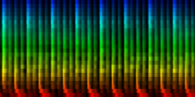
First up are the average classes.
| ||||
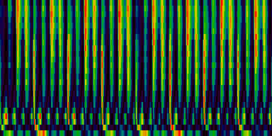
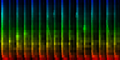
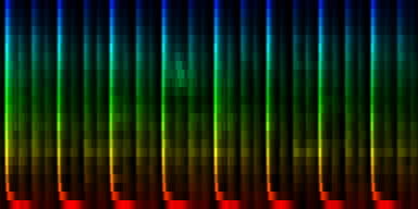
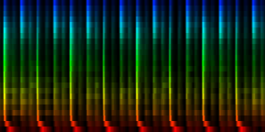
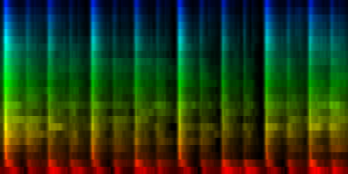
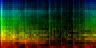
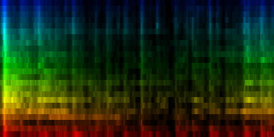
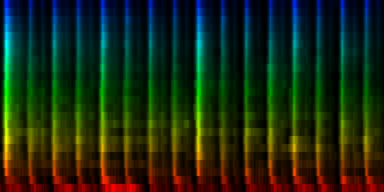
| The slow and fast average classes. The intensity reflects the presence of this energy at the specified time (horizontal) and frequency (vertical). The saturation of the color reflects the absolute deviation form the mean accross all provided samples. So, areas that are white are present in the average, but have a large deviation |
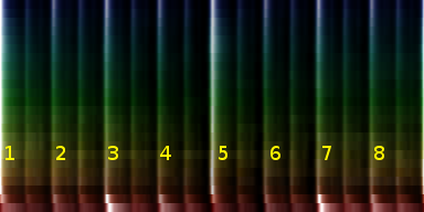
From the above picture we can already conclude a number of things. Beat number 1 and 5 are both present in the fast and slow class. So the chance that we could use that as a classification basis is unlikely. Certainly so, because the variance at beat 1 and 5 is relatively high.
Although the variances are low for 2, 3, 4 and 6, 7, 8 in the slow class, the variances for these beats are high in the fast class. So those are not very likely to be useful either.
The ticks between two beats, are much more stably present (lower absolute deviation), but since they tend to be present in slow and fast rhythms, the chance of finding a predictor here is also slim.
What we do however see is that 1/4th beats is much less present in the slow class. However, the energy is still present and one must then look at the empty spaces instead of the energy containing spaces.
As a side observation it is useful to note that the bassdrum in the slow class tends to be 'deeper'. Longer lasting, which is not a surprise since low tempos would sound a bit silly with a bassdrum of 100milliseconds, while one beat would last 1000ms.<
Potential avenues
- Look into the length of the average bassdrum. That seems somehow to relay to class.
- Look into the empty spaces between 1/4th beats. If there are empty areas, we might find an answer
- The presence of 1/4th beat hi hats might also be an indicator
Offset/Frequency positions with predictive Power
To measure the predictive power, we are not interested in the two-way correlation (that is whether 1 variable influences the other or not), but rather in whether the energy intensity at a certain position can say something about the class label (and to turn it upside down; we are not interested at all in the reverse: Whether the class label can say something about the energy we expect, although we already generated such a map).
To obtain the predictive power of a specific offset/frequency, we aggregated for that position, all energy intensities for both classes. That means, that we would for the slow class create a probability distribution of the energy within that class. For the fast class we would do exactly the same. Afterward, we would compare these two probability distributions between the classes and look for a threshold that would be the best differentiator between the two classes.
The differentiation is calculated based on the absolute difference between the both cumulative distributions. That in itself is merely a matter of walking through the sorted values of both distributions and reporting the maximum distance the two indices are separated.
What is finally reported is a threshold that gives us the probability difference cross the threshold. For instance, if the reported predictive power is 100%, then given that threshold, we can be 100% sure that the particular sample belongs to one class if it is above the threshold. If the predictive power is 50%, then we know that we have a 50% better chance if we prefer one class over another, to be correct.
| ||||
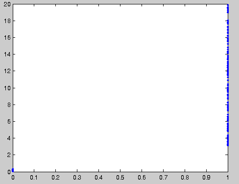
| In each of these figures, one sees the probability distributions of a two classes. (The slow class is for instance red, and the fast class could be green). To decide on the predictive power between those two classes, we create first the cummulative distribution. This can be found in the second row. These cmmulative probabilities are then subtracted (the graph in blue). In this blue graph we find the proper treshold where we have the maximum difference between the probability distributions. In the figure left, we could choose any treshold between 20 and 60. This treshold will ensure a perfect decission on the actual class. In the second graph, we can choose a treshold between 35 and 60. |
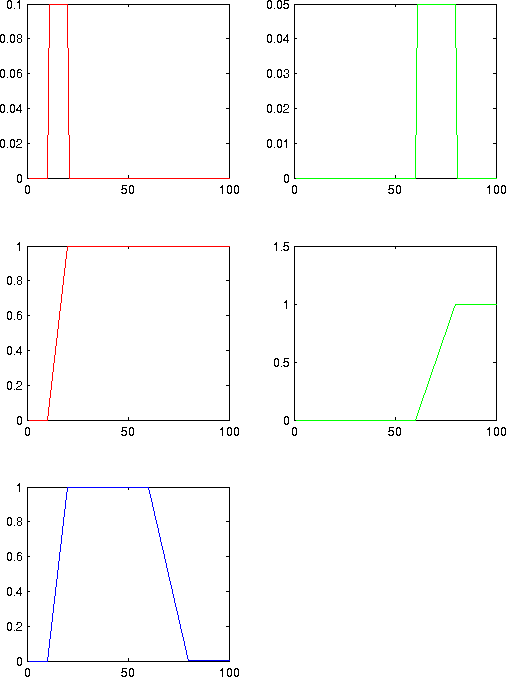
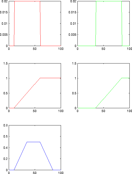
To understand this 'probability difference', it is useful to look at the above figure. Suppose that we would choose a threshold of 50 for the right figure, then we would have the following cross table
- If the class is slow, then
- 80% of the observed values will fall below the threshold
- 20% of the values will fall above the threshold
- If the class is fast, then
- 30% of the observed values will fall below the threshold
- 70% of the observed values will fall above the threshold
To jump from this observed probabilities to a preference to choose the class with the highest probability is not far fetched, except if you start to think about the frequencies of slow vs fast songs. In that case we must normalize these distribution. E.g: 30% of 1000 songs is still more than 80% of 10 songs. However, as already explained in the introduction. We do not want to bias ourselves towards the frequency of the underlying classes and as such we ignore the present frequencies.
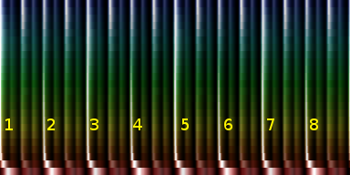
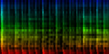
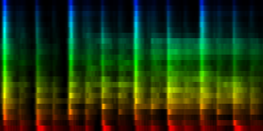
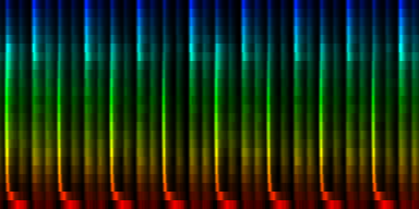
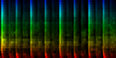
 Areas in a rhythmical pattern that are good differentiators between the slow and fast class. The hue and value are both reflecting the maximal difference between the cummaltive distribution of each class. The maximum value is 0.59 at red areas.
|
[Bootnote on correlations]
An avenue that one might consider now is whether a correlation measure could be useful. That is not the case because one variable (the class number) has only two potential values: 0 or 1. In this section I'd like to point out the following deficiency of the correlation coefficient.
In the simulated scenario we created a dataset that would for class 0, have 34 points between 0 and 0.3 (no energy essentially), and for class 1, we would have 138 points between 3 and 20. With two such distributions it is perfectly possible to predict the class based on the value. The only thing one needs to do is to check whether the value is larger than 1 (if so it is class 1) or not (in which case it is class 0). However, the correlation coefficient is calculated as 0.69 ! A very dissatisfying result. The matlab code follows:
C1X=random('unif',3,20,138,1);
C1Y=repmat(1,138,1);
C0X=random('unif',0,0.3,34,1);
C0Y=repmat(0,34,1);
X=[C0X; C1X];
Y=[C0Y; C1Y];
plot(Y,X,'.');
corr(X,Y)
 Horinzontally the class is shown (0 or 1). Vertically the energy distribution within that particular class. A cutoff of 1 will perfectly decide the proper class. However, the correlation coefficient of these two variables is 0.69
|
Normalisations
The topic of rhythmical normalisation has already been discussed in great detail in [2]. There are however a number of elements that will be used throughout this paper
- cut-mean - is the technique where we for each frequency band find the mean energy and subtract from each entry this mean (effectively bringing the mean to 0). Secondly, everything below 0 is removed and then the mean is calculated again and normalized to 1 (which effectively normalizes the variance to 1)
- normalize-mean brings the mean of each frequency band to 1 through division by the original mean. The variance is not normalized.
- without-echoes is a technique that finds the peaks in the beatgraph and will only place events at places where we have a large energy presence. This technique removes sound color and echoes completely
- quantile normalization This technique is the same as described in paper [2] except that each class has been weighted individually, which resulted in a target probability distribution that was not affected by the individual size of the classes.
Self Organizing Maps
Self organizing maps are based on a number of neurons (called
units), that will be treated to have an affinity to a specific
class. An excellent introduction to this approach can be found at
[3].
Initialisation
The initialization of such a network can be challenging. Certainly if we do not apply a distance function to smooth out a pattern and place it at many positions in the grid. In that case the choose of starting vectors is crucial. We tried the use of 0, but that would lead to all patterns being classified in 1 unit (because that one was closer to any pattern than the 0 vector was). We tried the use of the mean value (which worked, but it also biased the outcome towards the initial chosen elements). Then we experimented with a mean of 1 and a decreasing variance throughout the units. That worked better. And in the end we tried an approach where we would find the most distant elements in the dataset. The idea behind this is that we would select one element of the dataset and then look for the element that was furthest away from it. Based on these two elements we would start looking into the element that was then furthest away. Needless to say: if we worked with many units we would find that the initialization of the network was quite time consuming.
printf("Preparing unit %d\n",i);
for(int j = 0 ; j < floats_per_pattern; j++)
  u[j]=0;
if (i==0)
  for(int j = 0 ; j < n; j++)
    for(int k = 0 ; k < floats_per_pattern; k++)
      u[k]+=patterns[j][k]/n;
 else
   {
     double bD=0;
     int bU=0;
     for(int j = 0 ; j < n; j++)
       {
	 double D=0;
	 for(int k = 0 ; k < i; k++)
	   {
	     double d;
	     for(int l = 0 ; l < floats_per_pattern; l++)
	       d+=fabs(patterns[j][l]-U[k][l]);
	     D+=d*d;
	   }
	 if (D>bD)
	   {
	     bD=D;
	     bU=j;
	   }
       }
     memcpy(u,patterns[bU],bytes_per_pattern);
   }
U[i]=u;
The results of this approach were also somewhat unsatisfactory, so we started to use the distance function properly.
The output of 8 units
Below I show the results of the self organizing map when we present it with 1900 different songs
Unit  Counts  Slow  Fast
0     1414    0     395
1     480     2     4
2     1249    31    241
3     506     26    3
4     2417    261   387
5     746     19    59
6     2198    13    428
7     990     2     60
With cut-mean normalization
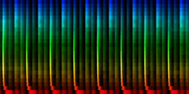
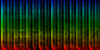
| ||||||||||||||||
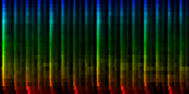
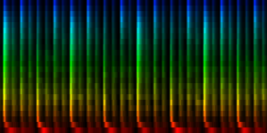
| 8 Patterns generated through a self organizing maps when the cut-mean normalization method is used. |
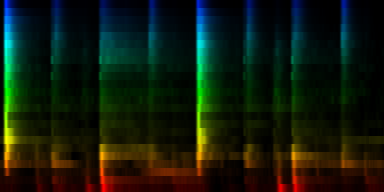
The interesting thing on these patterns is 'pattern 2'. That rhythm is a 3/4 measure which leaves room for some unexpected rhythms.
With ratio-mean normalization
Unit    Counts  Slow   Fast
0       554     6      36
1       1864    5      467
2       1204    0      494
3       1322    31     124
4       1435    15     235
5       2338    222    338
6       762     73     20
7       521     2      0
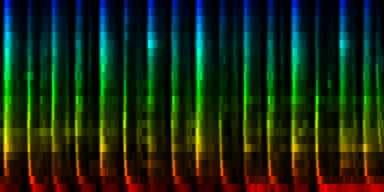
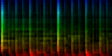
| ||||||||||||||||
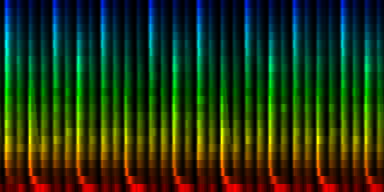
| 8 Patterns generated through a self organizing maps when the ratio-mean normalization method is used. |

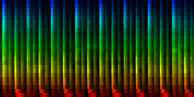
From these experiments it is not entirely clear which normalization method might yield the best results. We find that the normalize-mean patterns have less noise -if they had sufficient input data. This is to be expected since we did not arbitrarily set a cutoff value at the mean, so we did not introduce a discontinuity. We did however find that certain units (7) did not always attract sufficient information and we would in a sense waste 12.5% of out total computing time and resources on a useless neuron. That is highly unwanted.
Secondly, since we offer the self organizing map a lot more data than with the cut-mean method, it will also cluster in accordance with this extra data. We see this on the similar patterns that have mainly difference in accents. Oddly enough it is no longer able to find the 3/4 rhythm.
The amount and choice of normalization does matter. In particular, the cut-mean variant will normalize the highest energy to be 1, while the normalize_mean will not do such a thing and the highest energy could be anything. Because this later on might interact with the max_front algorithm, we might tend to favor the cutmean method since it normalizes the sound color and places all maximum to the same value of 1.
With min-max normalization
Unit    Counts  Slow   Fast
0       2254    2      350
1       1127    71     161
2       1402    0      386
3       864     0      247
4       761     78     39
5       1012    61     228
6       1465    140    95
7       1115    2      224
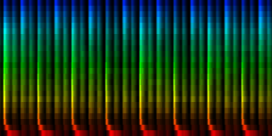
| ||||||||||||||||
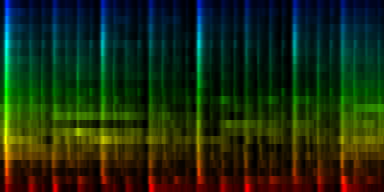
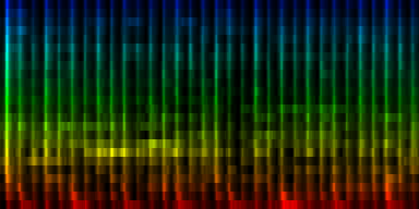
| 8 Patterns generated through a self organizing maps when the normalize-mean normalization method is used. |
In this result we don't see that much variation between the patterns, which is probably due to a selection against the sound color instead of the rhythm itself.
From these tests we can conclude that the cutmean variant is probably one of the better strategies.
With quantile normalization
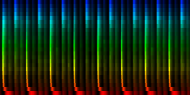
Unit    Counts  Slow   Fast
0       2435     0     269
1       1119     46    78
2       758      34    30
3       654      30    25
4       1257     6     238
5       1570     4     164
6       684      1     22
7       1523     39    66
-----------------------------
Success of testset: 84
Success when song is fast: 94
Success when song is slow: 38
| ||||||||||||||||
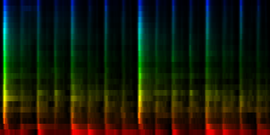
| 8 Patterns generated through a self organizing maps when the quantile normalization method is used. |
Weighing the map
One of the uses of the self organizing map is to test whether there can be a relation between the type of music and the slow/fast class. Although we expect this, it is not entirely clear whether such division is natural given our patterns. In order to test this question we started to cluster data with ever more units.
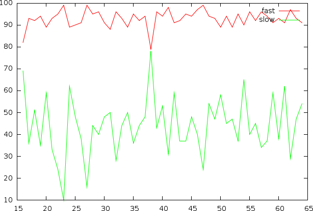 The efficiency of the various classes, once labeled, to report the proper outcome of a sample from the testset
|
From this graph we can conclude that there is a potentialto find some means of classifying slow versus fast rhythms. The problem however is that we might be offering the network the wrong type of data. As we already discovered during the univariate analysis, there is not much reason to look at the fronts of the 1st and 5th beat. Because these fronts contain more energy than other areas, it seems to become natural to remove these areas that we do not expect to have any predictive power.
In this approach we self-organized the output based on the predictive power coefficients as calculated in the univariate model, thereby relying on quantile normalization of the different frequency bands.
Unit    Counts  Slow    Fast    Slow    Fast    Successrate
0       857      48      23      56      21      72
1       886      15      37      18      39      68
2       1272      31     155      40     143      78
3       2453       1     150       0     161     100
4       1376       1     288       0     295     100
5       567       1       0       0       0       0
6       1566       6     168       2     174      98
7       1023      57      71      76      62      44
Success of testset: 85
Success when song is fast: 97
Success when song is slow: 29
Flux based measurements
One of the observations we made studying the differences between the two classes (slow versus fast), was the presence of a tail behind 16th notes that was not present in 32th notes. From this one could conclude that the energy flux might form a sensible predictor for this type of problem. Consequently, we created a flux based predictor that would measure the minimum and maximum energy for each window of a 16th, 32th and 64th note and then set out the probability distributions for the slow and fast class.
The first results were encouraging, in the sense that we were able to clearly see the difference between the distributions. When we then used a threshold to decide whether something was fast or slow, we found a positive result in 87% of the cases. 7.4 % of the slows songs was measured wrongly and 21.7 % of the fast songs was measured wrongly. This positive result could however not be transposed to the Dortmund dataset, in which we scores 92% of the fast ones wrong with the determined threshold.
The main reason of this failure is very likely the biased nature of the dataset. After all we have much more Goa trance than other music
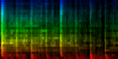
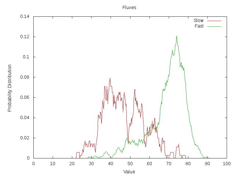 The flux distributuion for each category of songs
|
Conclusions
We must reconsider the idea that the rhythmic information is the sole source to classify music into slow or fast. Although the idea stems from 'tapping the tempo' and finding the beat, the natural extension to rhythm classification does not work. In general, there are rhythms that can be played fast as well as slow and for which the rhythmical pattern as such does not offer much useful information.
A strategy in which we used the univariate relations to create a Bayesian classifier did not work at all. We achieved only an overall 63% accuracy on the Dortmund selected set.
Future Work
Because it has become clear that the trainingset leads to a substantial bias in our experiments, we need some strategy to 'unbias' it.
Bibliography
| 1. | Biasremoval from BPM Counters and an argument for the use of Measures per Minute instead of Beats per Minute Van Belle Werner Signal Processing; YellowCouch; July 2010 http://werner.yellowcouch.org/Papers/bpm10/ |
| 2. | Rhythmical Pattern Extraction Werner Van Belle Signal Processing; YellowCouch; August 2010 http://werner.yellowcouch.org/Papers/rhythmex/ |
| 3. | Kohonen's Self Organizing Feature Maps unknown http://www.ai-junkie.com/ann/som/som1.html |
| http://werner.yellowcouch.org/ werner@yellowcouch.org |  |