| Home | Papers | Reports | Projects | Code Fragments | Dissertations | Presentations | Posters | Proposals | Lectures given | Course notes |
|
|
An Adaptive Filter for the Correct Localization of Subimages: FFT based Subimage Localization Requires Image Normalization to work properlyWerner Van Belle1* - werner@yellowcouch.org, werner.van.belle@gmail.com Abstract : How to find subimages with the fast fourier transform ? It is well documented how Fourier transforms can speed up image alignment. The cross-correlation of an image can be calculated as the inverse Fourier transform of the inproduct of the Fourier transform of the first image and the conjugated Fourier transform of the second image. However, when one tries to extend this useful relation to locate subimages in larger images we find that it no longer performs properly. In this document we describe a fast normalization method that makes it possible to use the standard Fourier based cross-correlation technique for subimage localization. The technique relies on a low pass filtering followed by an adaptive contrast enhancement.
Keywords:
Fourier transform FFT, cross correlation crosscorrelation phase correlation subimage finding subimage localization |
Table Of Contents
Introduction
In this article we first explain how Fourier transforms can be used to align two images of the same size. Afterwards we focus on the problem of subimage localization. To solve the problem of subimage localization we look into a normalization technique and finally combine this with a standard SAD matching algorithm to solve the subimage localization problem efficiently.
Cross Correlation
If we have two images A and B then the cross-correlation image C is defined as
If in the above equation (eq. 1) A and B are normalized based on their mean and standard deviation
then C reflects the true linear Pearson correlation at each potential translation.
The position ![]() where
where ![]() is maximal
determines the necessary translation to have the best overlap between
both images. The image
is maximal
determines the necessary translation to have the best overlap between
both images. The image ![]() is
sometimes written as
is
sometimes written as ![]() in which
in which
![]() can be read as a convolution
operation.
can be read as a convolution
operation.
Numerical Example
In the following we work with two small ![]() images. Calculating
images. Calculating
![]() shows that the best
translation between the two images is no
translation since the largest correlation value is found at position
shows that the best
translation between the two images is no
translation since the largest correlation value is found at position
![]() .
.
0       0       0        0
0       1       0        0
0       0       0.498039 0
0       0       0        0
0       0       0        0
0       1       0        0
0       0       0.498039 0
0       0       0        0
1.24804 0       0       0
0       0.49803 0       0
0       0       0       0
0       0       0       0.498039
When ![]() then the cross-correlation
is called autocorrelation.
then the cross-correlation
is called autocorrelation.
Fourier Based Implementation
The cross-correlation, defined as ![]() (eq. 1) is
an operation that, if implemented naively results in
(eq. 1) is
an operation that, if implemented naively results in ![]() operations. If we use a Fourier transform on both images we are able
to obtain a substantial speedup
operations. If we use a Fourier transform on both images we are able
to obtain a substantial speedup
A Fourier transform takes around ![]() operations, combined with the conjugation, inproduct and finding of
the maximum value, this results in a total calculation time of around
operations, combined with the conjugation, inproduct and finding of
the maximum value, this results in a total calculation time of around
![]() operations.
operations.
The above is well known and many examples can be found online. It is sometimes called phase correlation, although that name seems more fancy than providing useful understanding.
Numerical Example
To expand on the example given in section 1.1.1,
we calculate the Fourier transform of ![]() and
and ![]() ,
multiply them with each other and perform the backward transform
,
multiply them with each other and perform the backward transform
| FFTW | matlabs' fft2(X) |
0.37451 0 -0.12451 -0.25 -0.12549 0 -0.12451 -0.25 -0.12549 0 -0.12451 0.25 -0.12549 0 -0.12451 0.25 |
1.4980 -0.4980 - 1.0000i -0.5020 -0.4980 + 1.0000i -0.4980 - 1.0000i -0.5020 -0.4980 + 1.0000i 1.4980 -0.5020 -0.4980 + 1.0000i 1.4980 -0.4980 - 1.0000i -0.4980 + 1.0000i 1.4980 -0.4980 - 1.0000i -0.5020 |
| FFTW | matlabs' fft2(Y) |
0.37451 0 -0.12451 -0.25 -0.12549 0 -0.12451 -0.25 -0.12549 0 -0.12451 0.25 -0.12549 0 -0.12451 0.25 |
1.4980 -0.4980 - 1.0000i -0.5020 -0.4980 + 1.0000i -0.4980 - 1.0000i -0.5020 -0.4980 + 1.0000i 1.4980 -0.5020 -0.4980 + 1.0000i 1.4980 -0.4980 - 1.0000i -0.4980 + 1.0000i 1.4980 -0.4980 - 1.0000i -0.5020 |
| FFTW | fft2(X).*conj(fft2(Y)) |
0.140258 0 0.0780027 0 0.0157478 0 0.0780027 0 0.0157478 0 0.0780027 0 0.0157478 0 0.0780027 0 |
2.2441 1.2480 0.2520 1.2480 1.2480 0.2520 1.2480 2.2441 0.2520 1.2480 2.2441 1.2480 1.2480 2.2441 1.2480 0.2520 |
1.24804 0       0       0
0       0.49803 0       0
0       0       0       0
0       0       0       0.498039
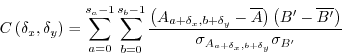
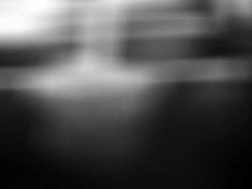
Image Example
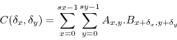
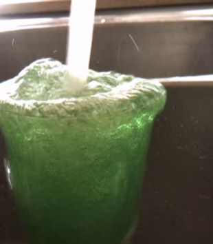
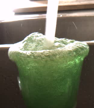
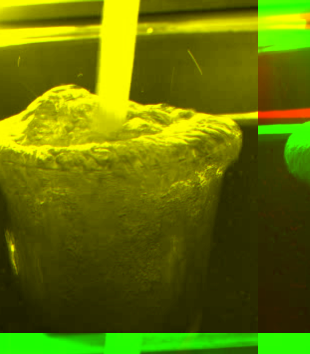
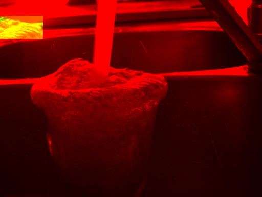
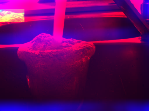
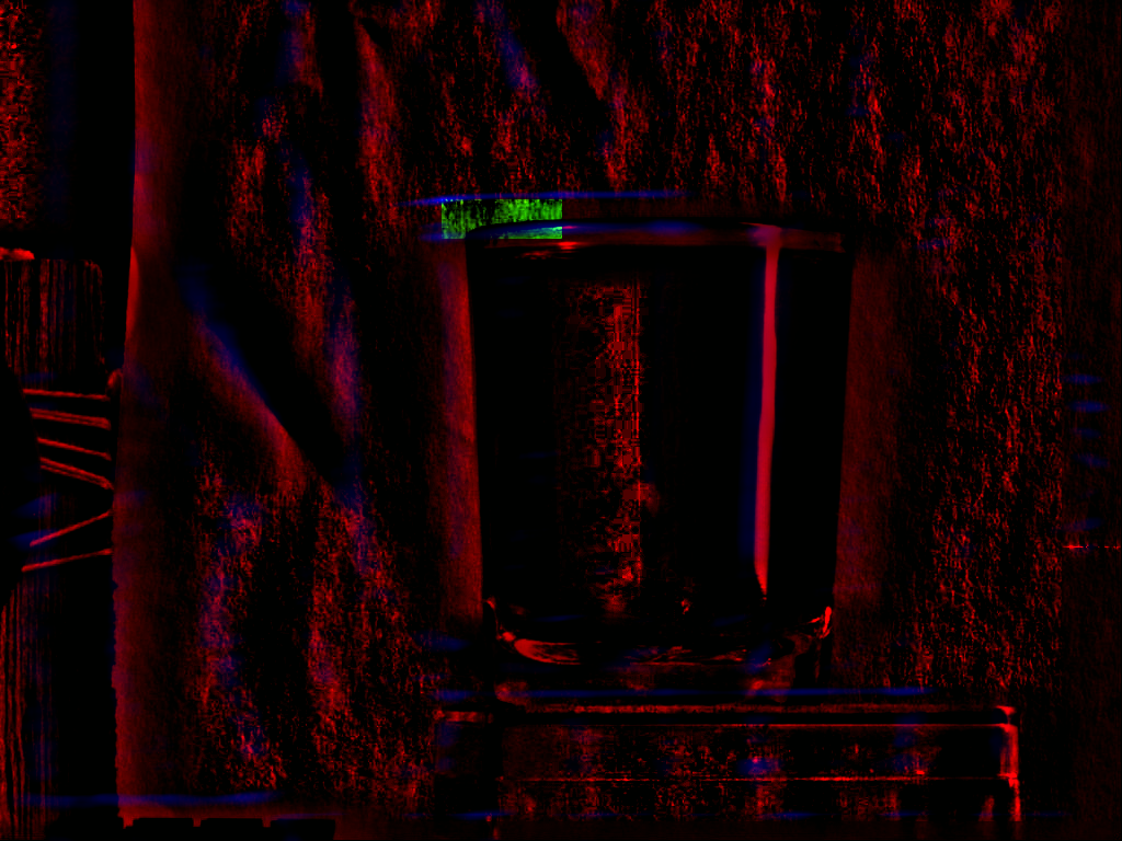
Figure 1 has two very similar
images
that ought to be aligned. After using the crosscorrelation algorithm
we obtain a correlation image that has a maximum value at ![]() ,
which is found in the image at the bottom right. Figure 2A
is the correlation strength map. Figure 2B
is the
superposition of the two images using two different channels. Red
is the first image. Green is the second image. Yellow areas are those
where both the red and green channels are present.
,
which is found in the image at the bottom right. Figure 2A
is the correlation strength map. Figure 2B
is the
superposition of the two images using two different channels. Red
is the first image. Green is the second image. Yellow areas are those
where both the red and green channels are present.
|
|
Code
The following code illustrates how to implement such an image alignment using using the FFTW library in C. The code requires Qt4 to read / write the images.
We assume that a and b are the images to be aligned, both have the same width and height. The fast fourier transform is the FFTW with the specialized r2c and c2r functions, meaning that we must take great care of the number of columns and rows present.
int ncols = a.width();
int nccols = ncols/2+1;
int nrows = a.height();
We allocate 4 arrays. The first is the amplitude of the original image a (Aa). The second is the amplitude of the second image (Ba). The third one is the amplitude of the cross correlation (Bc). Bf is the frequency representation of Aa and Af is the frequency representation of Aa.
double * Aa = (double*)fftw_malloc(sizeof(double)*ncols*nrows);
fftw_complex * Af = (fftw_complex*)fftw_malloc(sizeof(fftw_complex)*nccols*nrows);
double * Ba = (double*)fftw_malloc(sizeof(double)*ncols*nrows);
fftw_complex * Bf = (fftw_complex*)fftw_malloc(sizeof(fftw_complex)*nccols*nrows);
double * Bc = (double*)fftw_malloc(sizeof(double)*ncols*nrows);

fftw_plan forwardA = fftw_plan_dft_r2c_2d(nrows,ncols,Aa,Af,FFTW_FORWARD | FFTW_ESTIMATE);
fftw_plan backwardA = fftw_plan_dft_c2r_2d(nrows,ncols,Af,Aa,FFTW_BACKWARD | FFTW_ESTIMATE);
fftw_plan forwardB = fftw_plan_dft_r2c_2d(nrows,ncols,Ba,Bf,FFTW_FORWARD | FFTW_ESTIMATE);
fftw_plan backwardB = fftw_plan_dft_c2r_2d(nrows,ncols,Bf,Bc,FFTW_BACKWARD | FFTW_ESTIMATE);
Copy the images to the amplitude arrays and calculate Bf through the planned fftw.
for(int row = 0 ; row < nrows ; row++)
  for(int col = 0 ; col < ncols ; col++)
    Aa[col+ncols*row]=rgb2val(a.pixel(col,row));
fftw_execute(forwardA);
for(int row = 0 ; row < bsrow ; row++)
  for(int col = 0 ; col < bscol ; col++)
    Ba[col+ncols*row]=rgb2val(b.pixel(col,row));
fftw_execute(forwardB);
Multiply the frequency content of the first image with the conjugate
frequency content of the second image. Beware: complex multiplication
double norm=sqrt(ncols*nrows);
for(int j = 0 ; j < nccols*nrows ; j++)
  {
    double a = Af[j][0]/norm;
    double b = Af[j][1]/norm;
    double c = Bf[j][0]/norm;
    double d = -Bf[j][1]/norm;
    double e = a*c-b*d;
    double f = a*d+b*c;
    Bf[j][0]=e;
    Bf[j][1]=f;
  }
fftw_execute(backwardB);
Find the peak value.
double mx = Bc[0];
int mxat = 0;
for(int j = 0 ; j < ncols*nrows ; j++)
  if (Bc[j]> mx)
     mx=Bc[mxat=j];
printf("Best translation is over (%d,%d) pixels\n",mxat%ncols,mxat/ncols);
The subimage problem
Up to now, we assumed that the sizes of the images were similar. In case they are not we we are mainly interested in finding the best position of the smaller image in the larger image. This is called subimage localization. A common technique is to extend the sub-image with zeros (called zero-padding) or the mean value of A or B until it has the same size as the largest image. If we try this approach we find that it does not provides any useful information.
Image Example
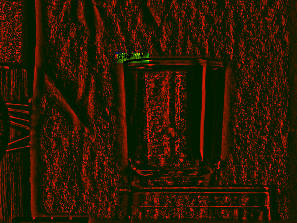
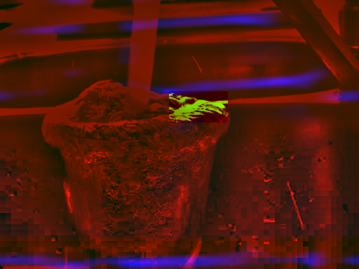
Figure 3 illustrates this on the
previous
image. The large image in this case is the entire image, while the
small rectangle designates the subimage we will try to find back in
the image. Figure 3B is the
correlation map
if we use the standard crosscorrelation algorithm. If we find the
maximum position in this correlation map we find that the coordinate
![]() is the optimal place to position the
subimage.
Figure 4 illustrates the positioning
of the
subimage on the larger image.
is the optimal place to position the
subimage.
Figure 4 illustrates the positioning
of the
subimage on the larger image.
|

|
As figure 3 illustrates, the correlation values seem wrong at many places. A closer investigation reveals that this is mainly due to the mean intensity throughout the image. The crosscorrelation calculates
If one of the two images has a larger mean then this will be reflected in the outcome of the sums and the crosscorrelation will reflect the mean intensity of the larger image. In other words, under the assumption that A and B had the same mean and variance this would have reflected the true linear Pearson cross-correlation. However, when we work with sub-images the assumption that the mean and variances are respectively 0 and 1 is not correct.
Numerical Example
As a numerical example of the problem we start with a large image
which has two patches of ![]() pixels. The first patch at the
top left all contains 1. The second patch (at position
pixels. The first patch at the
top left all contains 1. The second patch (at position ![]() ) alternates
between
) alternates
between ![]() and
and ![]() .
.
Larger Image
1      1       1       0       0       0       0       0
1      1       1       0       0       0       0       0
1      1       1       0       0       0       0       0
0      0       0       0       0       0       0       0
0      0       0       0       1       0.5     1       0
0      0       0       0       0.5     1       0.5     0
0      0       0       0       1       0.5     1       0
0      0       0       0       0       0       0       0
The alternating patch is the one we will be searching. To make a fourier transform possible we extend the 3x3 patch with zeros which gives
3x3 Subimage, zero-padded
1      0.5     1       0       0       0       0       0
0.5    1       0.5     0       0       0       0       0
1      0.5     1       0       0       0       0       0
0      0       0       0       0       0       0       0
0      0       0       0       0       0       0       0
0      0       0       0       0       0       0       0
0      0       0       0       0       0       0       0
0      0       0       0       0       0       0       0
Cross correlation
After cross correlation we find that the best match is found at position (0,0), this is logical because the multiplication of 1 with the subimage totals 7, while the multiplication of the subimage with itself only gives 6.
7     4.5     2.5     0       0       0       2.5     4.5
4.5   3       1.5     0       0       0       1.5     3
2.5   1.5     2       1       2.25    1       2       1.5
0     0       1       2.5     3       2.5     1       0
0     0       2.25    3       6       3       2.25    0
0     0       1       2.5     3       2.5     1       0
2.5   1.5     2       1       2.25    1       2       1.5
4.5   3       1.5     0       0       0       1.5     3
Towards a Solution
One might assume that padding the subimage with the mean of the larger image will provide a suitable normalization scheme. This however is incorrect since the positions where we actually are interested in a proper correlation (where the subimage has content), we still match against a potentially biased larger image (try it to find out !). So the only viable way forward is to keep on using zero padding since that is the only technique that will cancel out all the areas outside the subimage and use a suitable normalization scheme that works at a local level in the larger image.
Essentially, we are interested to calculate the real correlation between the subimage and the larger image for all potential translations. Assuming that a and b refer to coordinates in the subimage and that x and y refer to coordinates in the large image, we thus look for the largest value of C, where C is this time defined as
where ![]() is the subimage at position
is the subimage at position ![]() .
.
The problem now is that this new equation does not entirely fit to the original version of C. We can easily get rid of the areas surrounding the subimage A by setting the values outside A to zero. In that case we can change the summation range to go over the entire image. The places that fall outside the subimage A will become zero, regardless of the values for B.
The second consideration is that the mean we need to subtract from each image requires a preprocessing step, which is then followed by a normalization based on the standard deviation. When we combine these two steps we obtain a normalized image that sufficiently resembles the original equation C, and thus becomes usable in a Fourier transform setup.
The normalization of the images will use a) a lowpass filter to calculate the mean b) subtract the average from the original image, c) calculate the standarddeviation and d) normalize the standarddeviation. Each of these operations is dependent of a fast boxcar averaging, which can be implemented efficiently as follows.
Image Normalization
Fast lowpass filtering
To blur a 1 dimensional vector (a line or row from an image) through a specific windowsize, we work with two counters. The first keeps track of the total sum so far, the second keeps track of the amount of pixels actually involved in the current position. When we shift the sliding window to the right (or bottom in the 2nd dimension) we a) subtract the pixel going out of the window and b) add the pixel coming into the window. This make the lowpassfilter an O(n) operation regardless of the size of the window.
Code
double * blur(double *input, int sx, int wx)
  {
  double *horizontalmean = (double*)malloc(sizeof(double)*sx);
  double sum = 0;
  int count = 0;
  for(int x = 0 ; x < sx; x++)
    {
When we start (x==0) we initialize the counters by summing together
the entire sliding window.
    if (x == 0)
      for(int a = 0 ; a < wx; a++)
        {
        int c = x-wx/2+a;
        if (c < 0) continue;
        if (c >=sx) continue;
        sum+=input[c];
        count++;
        }
Otherwise, we shift the sum 1 to the right by removing the left pixel
and adding the right one.
    else
      {
      int c = x-1-wx/2;
      if (c >=0 && c < sx)
        {
        sum-=input[c];
        count-;
        }
      c = x+wx-1-wx/2;
      if (c >=0 && c < sx)
        {
        sum+=input[c];
        count++;
        }
      }
The mean is of course the sum of the entire window divided by the
current size of the window.
    means[x]=(double)sum/(double)count;
    }
Boxcar Averaging
To extend the above algorithm to 2 dimensions we merely perform the
linear time lowpass filter for each row, after which we execute the
lowpass filter for each column. The total time of the combined
operation
is. We annotate the mean image obtained through this method ![]() .
Figure 5 illsutrates this process
on the
grey values of the original image.
.
Figure 5 illsutrates this process
on the
grey values of the original image.
Variance Calculation
Once we have the mean image ![]() , we
can calculate the variance for
each pixel. This step takes the mean image calculated in section 3.2
and creates a new image
, we
can calculate the variance for
each pixel. This step takes the mean image calculated in section 3.2
and creates a new image ![]() ,
defined as
,
defined as
This image is then again averaged to obtain the variance in the
neighboorhood
of each position on the original image. The result is the variance
image, which we will call ![]() .
.
|
Code
int sx = input.width();
int sy = input.height();
int wx = atol(argv[3]);
int wy = atol(argv[4]);
double *img = (double*)malloc(sizeof(double)*sx*sy);
double *sqr = (double*)malloc(sizeof(double)*sx*sy);
for(int x = 0 ; x < sx ; x++)
  for(int y = 0 ;y < sy ; y++)
    img[x+y*sx]=qGray(input.pixel(x,y))/255.0;
double *mean = blur(img,sx,sy,wx,wy);
for(int j = 0 ; j < sx* sy ; j++)
  {
  double v = mean[j]-img[j];
  sqr[j]= v*v;
  }
double * var = blur(sqr,sx,sy,wx,wy);
Preparing the images
The last preprocessing step for the image is the subtraction of the
mean and division by the variance (when possible). In the code below
the fabs is necessary because the blurred version might sometimes
be a fraction lower than 0 due to roundoff errors (happens on fully
white images). The time complexity of this algorithm is ![]() for calculating
for calculating ![]() ,
, ![]() for calculating
for calculating ![]() ,
, ![]() for calculating
for calculating ![]() and
and ![]() for calculating the final
preprocessed
image. In total we thus have
for calculating the final
preprocessed
image. In total we thus have ![]() ,
which is independent of the size of the window.
,
which is independent of the size of the window.
Code
-
- for(int j = 0 ; j < sx* sy ; j++)
{
double v = sqrt(fabs(var[j]));
if (v<0.0001) v=0.0001;
img[j]=(img[j]-mean[j])/v;
}
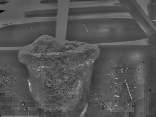
Image Example
|
Subimage Localization
Boundaries
The preprocessing of the subimage is slightly more complicated because we do not have enough information at the boundaries to have the same calculation of mean and variance as in the original image. In other words, if we have an image A from which we take an area B then we cannot normalize B such that normalizing A, and selecting the same area as B will give the same result.
Figure 8 illustrates two problems at the boundaries where the sliding window falls off the map. The first problem is numerical accuracy: calculating the standard deviation in a cumulative manner using floats is in general a bad idea. The second problem is that we have less information at the boundaries than at other positions in the image and we should start thinking of windowing the images.
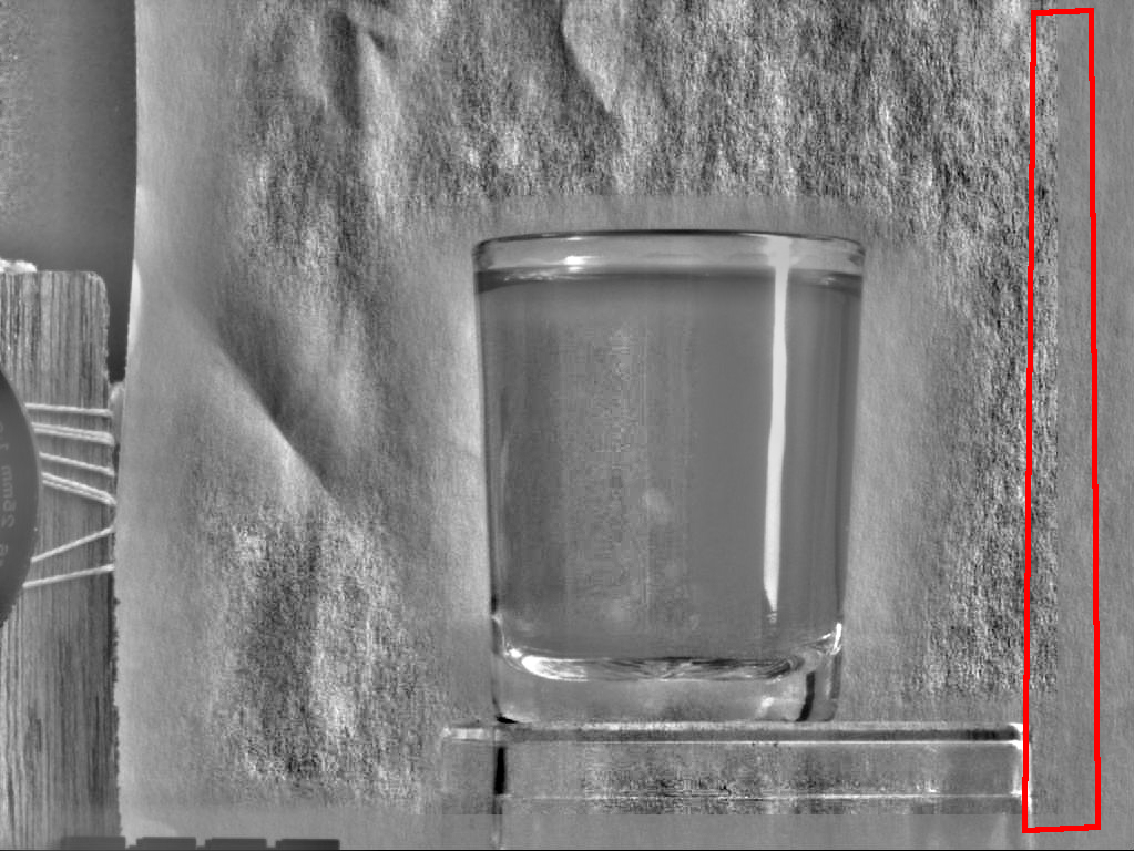
|
Window size
The importance of this problem is illustrated in figure figure 9. Depending on the window size we get different results.
|
Because a) the boundaries are important areas of errors in he correlation calculation and b) the window size is related to the accuracy of the results we must take care to darken the sides of the image based on the number of pixels included in that area. This results in a windowing of the subimage and if we want we could also apply it to the total image.
The normalization operation that includes the mean subtraction and
adaptive contrast enhancement as laid out in section 3
together with a darkening of the edges for the subimage will be called
![]() .
.
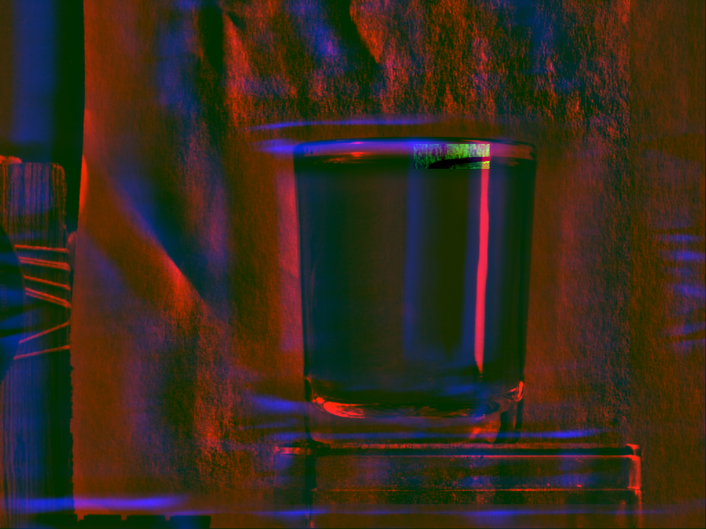
Localization
Based on the above example, we created two normalized images; one for the image in which we are looking for a specific pattern and one preprocessed pattern. Both operations can be performed in linear time compared to the image size and they both result in a matrix that has both positive as negative values. The resulting cross-correlation image will reflect the true linear Pearson correlation since both distributions (that of the image and the subimage) do have the same variances and means.
The full algorithm is described as
The optimal window size is the width of the subimage divided by 2 and the height of the subimage divided by 2. This makes sure we have a large area of the subimage that we take into account while still taking care of the boundary problems.
Remarkable with this algorithm is that this normalization scheme
leads to a less blurry correlation image as illustrated in figure 10.
Subimage finding through normalization of the images has a total time
complexity of ![]() .
.
|
Numerical Example
If we turn back to our numerical example from section 2.2, we find the following matrices after normalization:
0       0       1.22    -1.22   0      0       0      0
0       0       1.05    -1.12   0      0       0      0
1.22    1.05    1.76    -0.793  0      0       0      0
-1.22   -1.12   -0.793  -0.682  -0.60  -0.82   -0.62  -0.54
0       0       0       -0.609  2.3    0.003   2.15   -0.71
0       0       0       -0.825  0.003  0.492   0.003  -0.93
0       0       0       -0.626  2.15   0.003   1.97   -0.68
0       0       0       -0.544  -0.71  -0.938  -0.68  -0.62
1.03    -1.02    1.03
0        0       0
0        0      -1.02
 0.94  -0.09   1.04    0      0      0      1.04   -0.09
-0.09  -0.10   0.009   0      0      0      0.009  -0.1
 1.04   0.009  2.05   -0.5    1.54  -0.5    2.05    0.009
 0      0     -0.5     0.9   -1.57   0.9   -0.5     0
 0      0      1.54   -1.57   2.96  -1.57   1.54    0
 0      0     -0.50    0.90  -1.57   0.905 -0.502   0
 1.04   0.009  2.05   -0.50   1.54  -0.50   2.05    0.009
-0.09  -0.1    0.009   0      0      0      0.009  -0.1
which indeed reports the proper positioning. The fact that the correlation can be larger than 1 is because we did not divide the cross-correlation by the number of elements present in each vector.
The final step: SAD matching
|
The crosscorrelation matching described up to now works quite well
for many images. From a test set of 512 images, the matcher was able
to position a subimage correct in all but 8 of the images. A closer
investigation is the remaining errors revealed that crosscorrelation
is exactly what it states: it will calculate the crosscorrelation
between the subimage and the total image. Whether the ![]() norm is sufficiently small is not immediately contained within the
cross correlation results.
norm is sufficiently small is not immediately contained within the
cross correlation results.
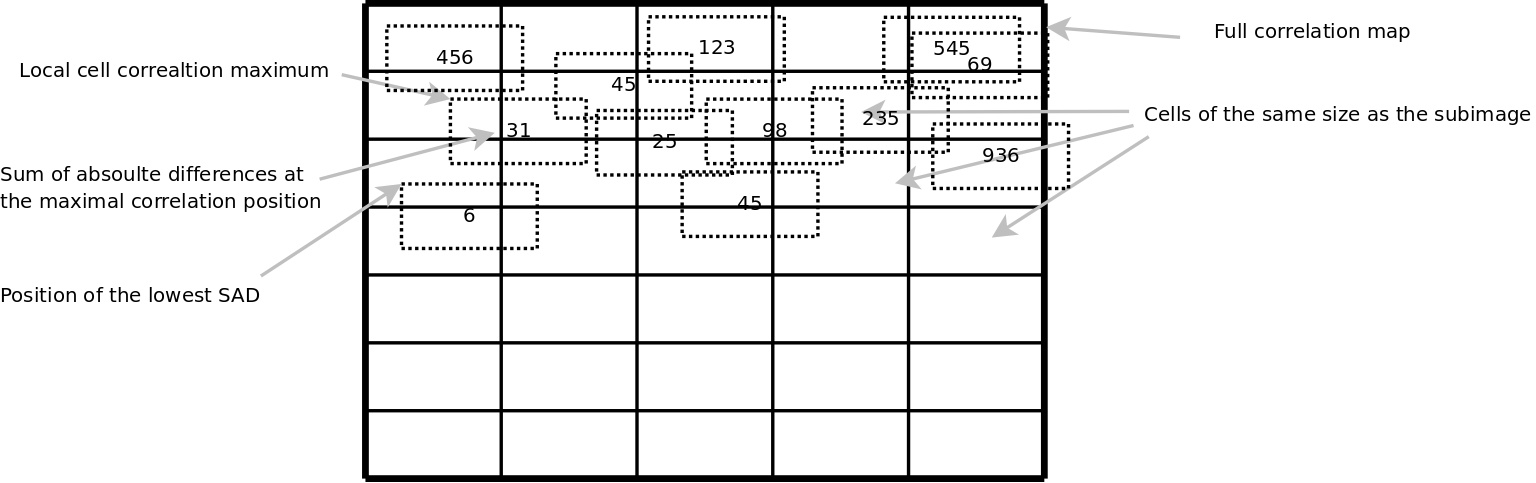
Therefore we extended the algorithm with a SAD grid matcher. The algorithm will essentially use the cross correlation image as a map together with a grid superimposed over the larger image. The cells in the grid are all the size of the subimage. In each cell we look for the best correlation and will for that position calculate the SAD. After calculation of all the SAD's of the better correlations will we report the coordinate with the lowest SAD.
Conclusion
We presented a normalization scheme suitable to find back subimages in larger images. The normalization is based on a hipass filter, an adaptive contrast enhancement and proper windowing before a standard FFT based cross correlation technique can be used. Based on the correctly calculated crosscorrelation map can we guide a sad-matcher (sum of absolute differences) to find the optimal position of the subimage in the larger image.
The full code can be downloaded here: subimg.c++.
The program was wrapped into a Perl module by Dennis Paulsen. See
http://search.cpan.org/dist/Image-SubImageFind/
Warning: Each input image must have an even number of pixels horizontally and vertically.
/**
 * A subimage finder (c) Werner Van Belle - 2007
 * mailto: werner@yellowcouch.org
 * License: GPL2
 */
#include <assert.h>
#include <qcolor.h>
#include <math.h>
#include <fftw3.h>
#include <qimage.h>
#include <qrgb.h>
#include <qapplication.h>
#include <iostream>
using namespace std;

typedef unsigned char unsigned1;
typedef signed short signed2;
typedef signed long long signed8;
signed2* boxaverage(signed2*input, int sx, int sy, int wx, int wy);
void window(signed2 * img, int sx, int sy, int wx, int wy);
signed2* read_image(char* filename, int& sx, int&sy);

void normalize(signed2 * img, int sx, int sy, int wx, int wy)
{
  /**
   * Calculate the mean background. We will subtract this
   * from img to make sure that it has a mean of zero
   * over a window size of wx x wy. Afterwards we calculate
   * the square of the difference, which will then be used
   * to normalize the local variance of img.
   */
  signed2 * mean = boxaverage(img,sx,sy,wx,wy);
  signed2 * sqr = (signed2*)malloc(sizeof(signed2)*sx*sy);
  for(int j = 0 ; j < sx * sy ; j++)
    {
      img[j]-=mean[j];
      signed2 v = img[j];
      sqr[j]= v*v;
    }
  signed2 * var = boxaverage(sqr,sx,sy,wx,wy);
  /**
   * The normalization process. Currenlty still
   * calculated as doubles. Could probably be fixed
   * to integers too. The only problem is the sqrt
   */
  for(int j = 0 ; j < sx * sy ; j++)
    {
      double v = sqrt(fabs(var[j]));
      assert(isfinite(v) && v>=0);
      if (v<0.0001) v=0.0001;
      img[j]*=32/v;
      if (img[j]>127) img[j]=127;
      if (img[j]<-127) img[j]=-127;
    }
  /**
   * Mean was allocated in the boxaverage function
   * Sqr was allocated in thuis function
   * Var was allocated through boxaveragering
   */
  free(mean);
  free(sqr);
  free(var);

  /**
   * As a last step in the normalization we
   * window the sub image around the borders
   * to become 0
   */
  window(img,sx,sy,wx,wy);
}

/**
 * This program finds a subimage in a larger image. It expects two arguments.
 * The first is the image in which it must look. The secon dimage is the
 * image that is to be found. The program relies on a number of different
 * steps to perform the calculation.
 *
 * It will first normalize the input images in order to improve the
 * crosscorrelation matching. Once the best crosscorrelation is found
 * a sad-matchers is applied in a grid over the larger image.
 *
 * The following two article explains the details:
 *
 *   Werner Van Belle; An Adaptive Filter for the Correct Localization
 *   of Subimages: FFT based Subimage Localization Requires Image
 *   Normalization to work properly; 11 pages; October 2007.
 *   http://werner.yellowcouch.org/Papers/subimg/
 *
 *   Werner Van Belle; Correlation between the inproduct and the sum
 *   of absolute differences is -0.8485 for uniform sampled signals on
 *   [-1:1]; November 2006
 */
int main(int argc, char* argv[])
{
  QApplication app(argc,argv);
  if (argc!=3)
    {
      printf("Usage: subimg <haystack> <needle>\n"
             "\n"
             "  subimg is an image matcher. It requires two arguments. The first\n"
             "  image should be the larger of the two. The program will search\n"
             "  for the best position to superimpose the needle image over the\n"
             "  haystack image. The output of the the program are the X and Y\n"
             "  coordinates.\n\n"
             "  http://werner.yellowouch.org/Papers/subimg/\n");
      exit(0);
    }

  /**
   * The larger image will be called A. The smaller image will be called B.
   *
   * The code below relies heavily upon fftw. The indices necessary for the
   * fast r2c and c2r transforms are at best confusing. Especially regarding
   * the number of rows and colums (watch our for Asx vs Asx2 !).
   *
   * After obtaining all the crosscorrelations we will scan through the image
   * to find the best sad match. As such we make a backup of the original data
   * in advance
   *
   */

  int Asx, Asy;
  signed2* A = read_image(argv[1],Asx,Asy);
  int Asx2 = Asx/2+1;

  int Bsx, Bsy;
  signed2* B = read_image(argv[2],Bsx,Bsy);

  unsigned1* Asad = (unsigned1*)malloc(sizeof(unsigned1)*Asx*Asy);
  unsigned1* Bsad = (unsigned1*)malloc(sizeof(unsigned1)*Bsx*Bsy);
  for(int i = 0 ; i < Bsx*Bsy ; i++)
    {
      Bsad[i]=B[i];
      Asad[i]=A[i];
    }
  for(int i = Bsx*Bsy ; i < Asx*Asy ; i++)
    Asad[i]=A[i];

  /**
   * Normalization and windowing of the images.
   *
   * The window size (wx,wy) is half the size of the smaller subimage. This
   * is useful to have as much good information from the subimg.
   */
  int wx=Bsx/2;
  int wy=Bsy/2;
  normalize(B,Bsx,Bsy,wx,wy);
  normalize(A,Asx,Asy,wx,wy);


  /**
   * Preparation of the fourier transforms.
   * Aa is the amplitude of image A. Af is the frequence of image A
   * Similar for B. crosscors will hold the crosscorrelations.
   */
  double * Aa = (double*)fftw_malloc(sizeof(double)*Asx*Asy);
  fftw_complex * Af = (fftw_complex*)fftw_malloc(sizeof(fftw_complex)*Asx2*Asy);
  double * Ba = (double*)fftw_malloc(sizeof(double)*Asx*Asy);
  fftw_complex * Bf = (fftw_complex*)fftw_malloc(sizeof(fftw_complex)*Asx2*Asy);

  /**
   * The forward transform of A goes from Aa to Af
   * The forward tansform of B goes from Ba to Bf
   * In Bf we will also calculate the inproduct of Af and Bf
   * The backward transform then goes from Bf to Aa again. That
   * variable is aliased as crosscors;
   */
  fftw_plan forwardA = fftw_plan_dft_r2c_2d(Asy,Asx,Aa,Af,FFTW_FORWARD | FFTW_ESTIMATE);
  fftw_plan forwardB = fftw_plan_dft_r2c_2d(Asy,Asx,Ba,Bf,FFTW_FORWARD | FFTW_ESTIMATE);
  double * crosscorrs = Aa;
  fftw_plan backward = fftw_plan_dft_c2r_2d(Asy,Asx,Bf,crosscorrs,FFTW_BACKWARD | FFTW_ESTIMATE);

  /**
   * The two forward transforms of A and B. Before we do so we copy the normalized
   * data into the double array. For B we also pad the data with 0
   */
  for(int row = 0 ; row < Asy ; row++)
    for(int col = 0 ; col < Asx ; col++)
      Aa[col+Asx*row]=A[col+Asx*row];
  fftw_execute(forwardA);

  for(int j = 0 ; j < Asx*Asy ; j++)
    Ba[j]=0;
  for(int row = 0 ; row < Bsy ; row++)
    for(int col = 0 ; col < Bsx ; col++)
      Ba[col+Asx*row]=B[col+Bsx*row];
  fftw_execute(forwardB);

  /**
   * The inproduct of the two frequency domains and calculation
   * of the crosscorrelations
   */
  double norm=Asx*Asy;
  for(int j = 0 ; j < Asx2*Asy ; j++)
    {
      double a = Af[j][0];
      double b = Af[j][1];
      double c = Bf[j][0];
      double d = -Bf[j][1];
      double e = a*c-b*d;
      double f = a*d+b*c;
      Bf[j][0]=e/norm;
      Bf[j][1]=f/norm;
    }
  fftw_execute(backward);

  /**
   * We now have a correlation map. We can spent one more pass
   * over the entire image to actually find the best matching images
   * as defined by the SAD.
   * We calculate this by gridding the entire image according to the
   * size of the subimage. In each cel we want to know what the best
   * match is.
   */
  int sa=1+Asx/Bsx;
  int sb=1+Asy/Bsy;
  int sadx;
  int sady;
  signed8 minsad=Bsx*Bsy*256L;
  for(int a = 0 ; a < sa ; a++)
    {
      int xl = a*Bsx;
      int xr = xl+Bsx;
      if (xr>Asx) continue;
      for(int b = 0 ; b < sb ; b++)
        {
          int yl = b*Bsy;
          int yr = yl+Bsy;
          if (yr>Asy) continue;

          // find the maximum correlation in this cell
          int cormxat=xl+yl*Asx;
          double cormx = crosscorrs[cormxat];
          for(int x = xl ; x < xr ; x++)
            for(int y = yl ; y < yr ; y++)
              {
                int j = x+y*Asx;
                if (crosscorrs[j]>cormx)
                  cormx=crosscorrs[cormxat=j];
              }
          int corx=cormxat%Asx;
          int cory=cormxat/Asx;

          // We dont want subimages that fall of the larger image
          if (corx+Bsx>Asx) continue;
          if (cory+Bsy>Asy) continue;

          signed8 sad=0;
          for(int x = 0 ; sad < minsad && x < Bsx ; x++)
            for(int y = 0 ; y < Bsy ; y++)
              {
                int j = (x+corx)+(y+cory)*Asx;
                int i = x+y*Bsx;
                sad+=llabs((int)Bsad[i]-(int)Asad[j]);
              }

          if (sad<minsad)
            {
              minsad=sad;
              sadx=corx;
              sady=cory;
              // printf("* ");
            }
          // printf("Grid (%d,%d) (%d,%d) Sip=%g Sad=%lld\n",a,b,corx,cory,cormx,sad);
        }
    }
  printf("%d\t%d\n",sadx,sady);
  /**
   * Aa, Ba, Af and Bf were allocated in this function
   * crosscorrs was an alias for Aa and does not require deletion.
   */
  free(Aa);
  free(Ba);
  free(Af);
  free(Bf);
}

signed2* boxaverage(signed2*input, int sx, int sy, int wx, int wy)
{
  signed2 *horizontalmean = (signed2*)malloc(sizeof(signed2)*sx*sy);
  assert(horizontalmean);
  int wx2=wx/2;
  int wy2=wy/2;
  signed2* from = input + (sy-1) * sx;
  signed2* to = horizontalmean + (sy-1) * sx;
  int initcount = wx - wx2;
  if (sx<initcount) initcount=sx;
  int xli=-wx2;
  int xri=wx-wx2;
  for( ; from >= input ; from-=sx, to-=sx)
    {
      signed8 sum = 0;
      int count = initcount;
      for(int c = 0; c < count; c++)
        sum+=(signed8)from[c];
      to[0]=sum/count;
      int xl=xli, x=1, xr=xri;
      /**
       * The area where the window is slightly outside the
       * left boundary. Beware: the right bnoundary could be
       * outside on the other side already
       */
      for(; x < sx; x++, xl++, xr++)
        {
          if (xl>=0) break;
          if (xr<sx)
            {
              sum+=(signed8)from[xr];
              count++;
            }
          to[x]=sum/count;
        }
      /**
       * both bounds of the sliding window
       * are fully inside the images
       */
      for(; xr<sx; x++, xl++, xr++)
        {
          sum-=(signed8)from[xl];
          sum+=(signed8)from[xr];
          to[x]=sum/count;
        }
      /**
       * the right bound is falling of the page
       */
      for(; x < sx; x++, xl++)
        {
          sum-=(signed8)from[xl];
          count--;
          to[x]=sum/count;
        }
    }

  /**
   * The same process as aboe but for the vertical dimension now
   */
  int ssy=(sy-1)*sx+1;
  from=horizontalmean+sx-1;
  signed2 *verticalmean = (signed2*)malloc(sizeof(signed2)*sx*sy);
  assert(verticalmean);
  to=verticalmean+sx-1;
  initcount= wy-wy2;
  if (sy<initcount) initcount=sy;
  int initstopat=initcount*sx;
  int yli=-wy2*sx;
  int yri=(wy-wy2)*sx;
  for(; from>=horizontalmean ; from--, to--)
    {
      signed8 sum = 0;
      int count = initcount;
      for(int d = 0 ; d < initstopat; d+=sx)
        sum+=(signed8)from[d];
      to[0]=sum/count;
      int yl=yli, y = 1, yr=yri;
      for( ; y < ssy; y+=sx, yl+=sx, yr+=sx)
        {
          if (yl>=0) break;
          if (yr<ssy)
            {
              sum+=(signed8)from[yr];
              count++;
            }
          to[y]=sum/count;
        }
      for( ; yr < ssy; y+=sx, yl+=sx, yr+=sx)
        {
          sum-=(signed8)from[yl];
          sum+=(signed8)from[yr];
          to[y]=sum/count;
        }
      for( ; y < ssy; y+=sx, yl+=sx)
        {
          sum-=(signed8)from[yl];
          count--;
          to[y]=sum/count;
        }
    }
  free(horizontalmean);
  return verticalmean;
}

void window(signed2 * img, int sx, int sy, int wx, int wy)
{
  int wx2=wx/2;
  int sxsy=sx*sy;
  int sx1=sx-1;
  for(int x = 0 ; x < wx2 ; x ++)
    for(int y = 0 ; y < sxsy ; y+=sx)
      {
        img[x+y]=img[x+y]*x/wx2;
        img[sx1-x+y]=img[sx1-x+y]*x/wx2;
      }

  int wy2=wy/2;
  int syb=(sy-1)*sx;
  int syt=0;
  for(int y = 0 ; y < wy2 ; y++)
    {
     for(int x = 0 ; x < sx ; x ++)
       {
         /**
          * here we need to recalculate the stuff (*y/wy2)
          * to preserve the discrete nature of integers.
          */
         img[x + syt]=img[x + syt]*y/wy2;
         img[x + syb]=img[x + syb]*y/wy2;
       }
     /**
      * The next row for the top rows
      * The previous row for the bottom rows
      */
     syt+=sx;
     syb-=sx;
     }
}

signed2* read_image(char* filename, int& sx, int&sy)
{
  QImage input((QString)filename);
  sx = input.width();
  sy = input.height();
  assert(sx>4 && sy>4);
  signed2 *img = (signed2*)malloc(sizeof(signed2)*sx*sy);
  for(int x = 0 ; x < sx ; x++)
    for(int y = 0 ;y < sy ; y++)
      img[x+y*sx]=qGray(input.pixel(x,y));
  return img;
}
| http://werner.yellowcouch.org/ werner@yellowcouch.org |  |