| Home | Papers | Reports | Projects | Code Fragments | Dissertations | Presentations | Posters | Proposals | Lectures given | Course notes |
|
|
An Experiment in Automatic Mastering.Werner Van Belle1 - werner@yellowcouch.org, werner.van.belle@gmail.com Abstract : This document describes an experiment in 'automatstering'. That is, mastering audiotool tracks with as little user input as possible. Allthough that experiment failed we learned a fair amount of interesting things along the ways. This is a writeup of a number of these things
Keywords:
matching equalizer, mastering, a-records |
Table Of Contents
Introduction
 Mastering pipeline
|
This document describes an experiment in 'automatstering'. That is, mastering audiotool tracks with as little user input as possible. Although that experiment failed we learned a fair amount of interesting things along the ways. This is a writeup of a number of these things. The master techniques described below have been used on the A-records 'Flowid' and 'Klub Affekt' releases.
A typical mastering pipeline involves equalization, stereo imaging, adding/removing dynamics, loudness enhancement, dithering, and mp3 compression. Below I will go into some of the details of each phase.
Obtaining the signal
Although a normal mastering pipeline would start working with individual tracks, in our case we started with a downmixed signal. Individual track extraction would take too much time and be too complicated, and could also not be performed automatically. E.g: think of an aux send with reverb and you'll quickly realize that a simple automatic selection of individual channels on the centroid might not be sufficient.
The downmixes were generated as floating point exports. Floats were chosen because they are not 'limited' to a certain dynamic range such as short integers are (They have a dynamic range of about 1529 dB, while integers have a dynamic range of 90 decibels). That means that we could turn of the limiter and simply write the data to disk. Whereas if we would do this with integers we would often get a distorted audio stream.
A second advantage of using floats is that they are not easily quantized. If the signal generated by audiotool is 0.000025 then an integer conversion would make a 0 out of this. And we would loose information. That is especially important since some artists placed the volume of their track sufficiently low such that it would not clip or push the limiter too much. However, that also meant that all instruments that fell below the transients already lost ~1 bit (6 dB, 6.666% of the total) dynamic range.
Aside from exporting, sometimes, when the artist applied too much compression himself we rendered the tracks without compressor. Equally so for artists placing a final equalizer before the outputbox (RNZR - why did you do that ?). In all cases, the limiter was turned off.
A last step to obtain the signal was to trim all empty space in front and behind the track.
DC Offset removal
With our signal in hand, we must first remove the DC-offset
DC offset refers to all frequencies below a certain threshold (for instance 30 Hz). An oscillation of 1Hz is considered a DC offset. It reduces the dynamic range of the signal and makes all other frequencies sound somewhat 'muddy', not clearly defined. DC offset removal is an important part to create a good sound and is necessary to reduce power consumption on old amplifiers.
Internally, audiotool generates a lot of 'DC offset'. Just set the Heisenberg to a low oscillation of 0 Hz and you create it. Also the pulverisateur seems to generate it without much hesitation.
To remove the DC offset, a high pass filter at low frequency (E.g 40 Hz) is applied. Sadly, often an inappropriate IIR filter [1] (high quality Butterworth [2] or so) is applied. This removes the DC offset but also makes each bass drum sound out of sync (which they indeed are then).
This can be solved by using a more expensive linear phase filter, which, as someone noticed on dsprelated [3], can be implemented quite efficiently using a stack of moving averages. The April 2012 update of audiotool introduced such DC limiter, so the signal received from audiotool no longer requires an individual step there and is already of higher quality than what some mastering tools provide.
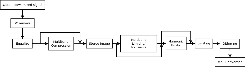
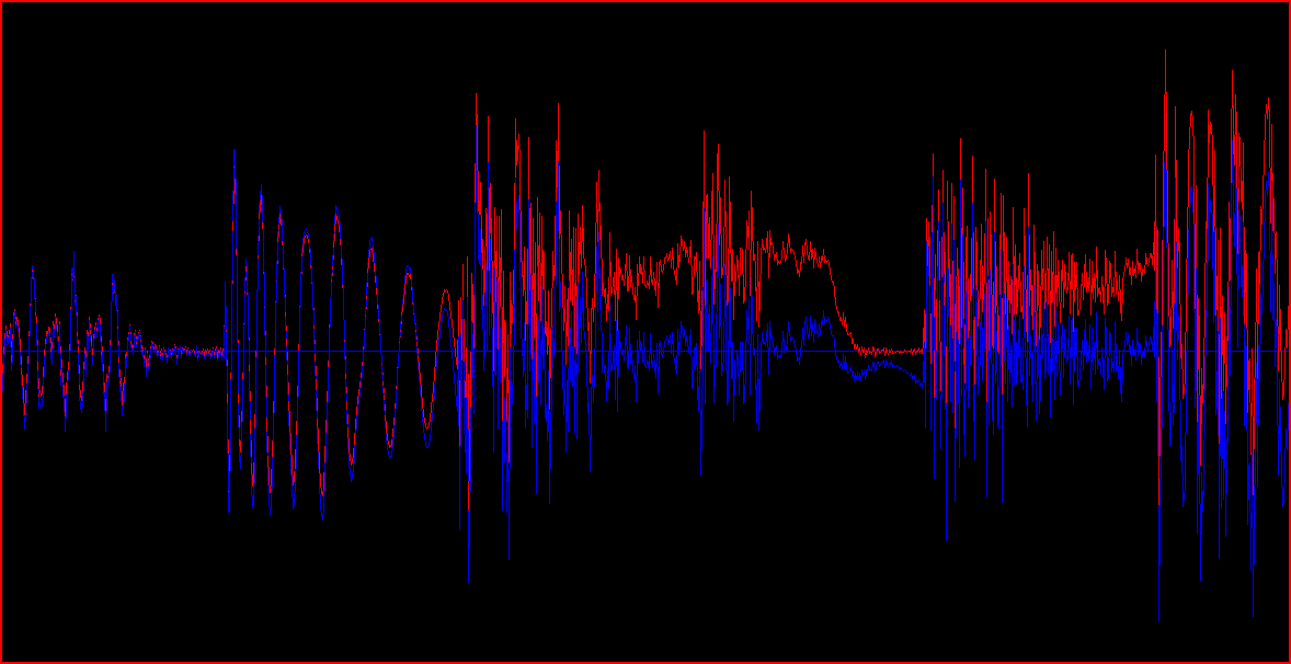 The red curve is the signal
coming out of the various synthesizers. The blue curve is after DC
removal
The red curve is the signal
coming out of the various synthesizers. The blue curve is after DC
removal
|
Equalizing
Tooling
Music equalization is a difficult topic and often the wrong tools are used to solve specific problems. For instance, one is easily tempted to use good old fashioned IIR filters [1] (Butterworth [2], biquad filters, shelving filter). The problem with these is that they delay one frequency more than the other and this is totally unacceptable for a high quality mastering; certainly so because nowadays nothing prohibits us to use linear phase FIR filters. They are a lot slower but nobody cares how long much time it takes to render a track.
The second problem is that most frequency tools show the spectrum at an instantaneous moment. This is of course cool (nice moving images), but it does not give an overview of what frequencies are 'on average' visible. To deal with that we created a tool that would scan the entire song, set up a histogram of the music and show us the median, 75 percentile, 87 percentile energy levels. We choose percentile measures because true averages in the statistical sense would be affected too much by outliers. E.g: the value at the 75th percentile is not much affected by how much empty space there is in the track.
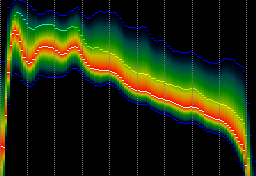 The energy distribution for a
typical audiotool song. From left to right the 10 octaves are
set out. Vertically the energystrength on a logarithmic (dB) scale. The color represents how often
this frequency energy was present in the song. Darkblue - seldom present. Intense red: often present.
The energy distribution for a
typical audiotool song. From left to right the 10 octaves are
set out. Vertically the energystrength on a logarithmic (dB) scale. The color represents how often
this frequency energy was present in the song. Darkblue - seldom present. Intense red: often present.
|
Using our tool we were able to
- investigate existing songs.
- modify the spectrum any way we wanted, using a high quality linear filtering.
- merge compression into equalizing
Equalisation target
When looking at well mastered songs, we generally saw linear slopes on an octave/db frequency plot. And of course this led to the realization to we could make the music fit such linear slope. Some tests later we figured out that this did not entirely work and that choosing a correct target depends on the style of music. Below I'll go into some detail of the various curves we investigated
Fletcher-Munson curve and the ISO226 target
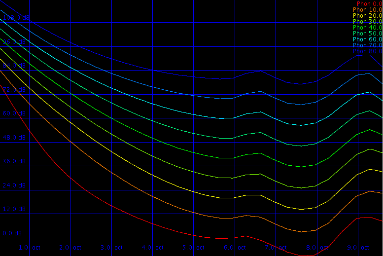 The ISO 226
Target. Horizontal the various octaves are set out. Vertically the
required decibelss to match a tone that was originally X phon at 1
kHz
The ISO 226
Target. Horizontal the various octaves are set out. Vertically the
required decibelss to match a tone that was originally X phon at 1
kHz
|
In the articles [4, 5, 6, 7], the aithors tested how people perceive music. They did this by placing a note at 1 KHz and then changing the frequency. Each listener had to modify the volume then to match the loudness of the 1 Khz tone. This resulted in a plot as shown above. Later on this experiment was repeated at a larger scale and produced pretty much the same curve. This experiment is widely criticized as not being 'believable' because 'at those times' it would have been impossible to generate such accurate signals without introducing distortion. A second criticism is that more than 40% of the people tested were Asian. We western people just don't really like that.
Another problem with these curves is that they deal with pure tones. Music is not a pure tone. They do however indicate us how loud a certain frequency might be to 'fit in the whole'.
Notwithstanding this criticism and the various drawbacks of those curves, some music sounded better if we used this as target.
BBC Loudness measurements and the ITU-468 curve
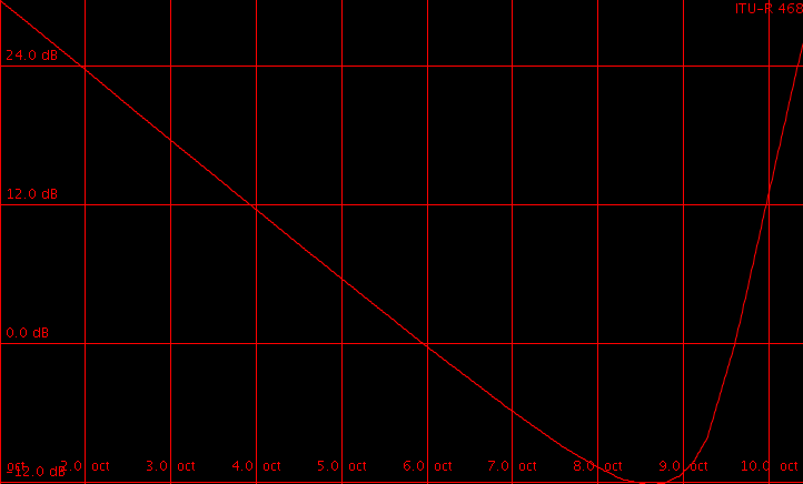 The ITU-468 loudness target
|
[8] describes a system to not only measure pure tones but takes into account bursts. They observed that a series of bursts will be perceived differently loud, when the frequency of the burst changes. As soon as a series of burst becomes tonal it lowers in loudness. To take this into account they created a half peak rectifier (a charging capacitor) with a decay time of about 150 milliseconds. That way they were able to measure loudness. Aside from that they also introduced an equalization curve that should be applied before measuring the loudness of a signal.
Currently this research has been transformed into the ITU-468 target [9]. One could assume that inverting the necessary equalization for loudness measurement would tell us something about the equalization target, visualized above'. Our experience using the ITU-468 curve is that it sometimes works quite well, other times it doesn't.
The EU Target
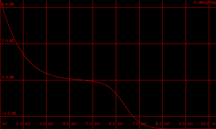 Loudness target based on K-weighting
from the EU EBU standard
Loudness target based on K-weighting
from the EU EBU standard
|
Of course regulatory bodies all need their own standard; and so did the EU. In 2011 they came up with a loudness measuring scheme [10, 11] that takes into account various time scales and also uses an equalization curve, K-weighting, which is just weird. Any test I conducted with this curve resulted in disaster. Probably I have been using that curve in a totally wrong context.
An average target
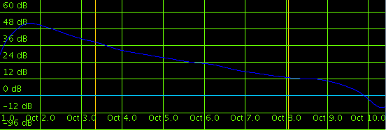 The average energy presence in
the Club-Affekt winning songs.
The average energy presence in
the Club-Affekt winning songs.
|
When mastering a CD containing multiple artists, there is another option that one could use. Instead of using a fixed target we can use the average spectrum of all songs on the CD, and use that as target to match for each individual song. After all, such compilation involves the best artists at audiotool, working each with their individual installation and their specific interpretation of sound. In a sense, by providing us with their music, they all tell us how the sound should be. By averaging their interpretation we obtain a very solid sampling of 'what is out there'.
We noticed when averaging multiple songs is that they tend to generate linear targets as well, except that they are properly bandlimitted, and otherwise substantially different from the theoretical estimates above. Our experience with this strategy was that it works better than any of the synthetic curves; although it is biased towards the style present on the CD.
Boundaries
In all of the above curves, one problem remained. Although we might need to play a tone at 22kHz 30 dB louder to have the same effect as a tone of 0dB at 1kHz; it really isn't a good strategy to indeed equalize the sound such that we boost those high frequencies so much. Similarly, some curves just extrapolate at the lower end of the scale and assume that at 0Hz, we need the signal to be 120 dB louder. Not a good idea either.
So, aside from using a suitable target, we must also specify from where to where we would like to apply that target. We need to specify the lowest frequencies that the artist accessed (typically the frequency of the bass drum) and the largest frequency where the artist placed musical content. The latter is of course more tricky to determine because, at the higher frequencies a lot of noise and garbage ends up. There we manually had to decide where the music stopped and the garbage started. Below the lower limit and above the higher limit we didn't modify the spectrum
Slant
A third parameter that we discovered when working with various music, is that, even after 'flattening out' the spectrum, one still had to apply a certain fall-off. With every increasing octave, the sound had to be lowered ~4.5dB. How steep this drop is determines how the sound is 'balanced between lo and hi. This was also manually done.
The A-records mastering
The balancing of the target-strength, slant, lo and hi boundaries is somewhat delicate and has been tuned manually for most songs. For instance, matching the target curve perfectly with a start octave a bit too low and a stop octave a bit too high, would make the sound 'great', until you saved it and listened to it the next day. Then it would sound 'hollow'. So at this stage we had to hack ourselves. We would master all tracks, wait until the next day. Listen to them again, fix problems. And repeat this process until the tracks were better than the original and sounded 'great' directly when opened.
One instance where this 'hollowing out' was wanted was our advertisment video. There we want to leave room for the artists voices.
For the flow mastering, we used the average target. Some tracks came out sounding slightly worse than the original (e.g: Grotzo); but when listening to them 'in the flow', they now fitted in much better.
For the Affekt mastering we used a different strategy. This time a meta-strategy was used to attain two goals 1) it should fit in the overall mood of the CD; 2) each individual track should be better than the original. To achieve this we mastered the CD 4 times. Each time with a different target. Once we mastered it with the average of the CD, once with the ITU-468 target and once with the ISO-226 target. A fourth time was necessary for some peculiar tracks that had completely different dynamics than other tracks (E.g. the rnzr track had almost no body in the bass drums and; compared to other tracks, was just a series of ticks and clicks. This skewed the measurement of the equalization and consequently the equalization we applied). For some tracks the result (Trancefreak12) was better than the original, but somewhat 'out of the possible wanted style' for that genre.
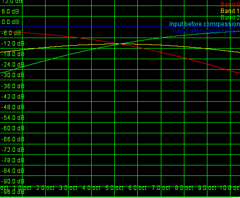
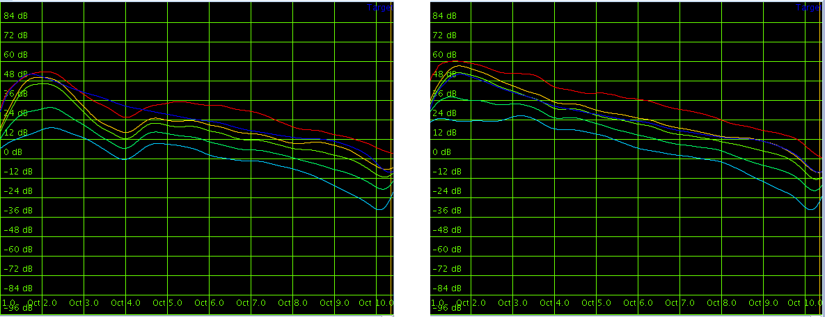 Frequency plots of
Perfoliate by Rnzr before and after equalizing.
Frequency plots of
Perfoliate by Rnzr before and after equalizing.
|
In the above audio fragment, the original is first, the equalized version is second. In this case the equalization target was the average sound of all tracks on the album.
Stereo image
A tricky problem when mastering manually is to set the levels of the left and right channel equally loud. I've never seen a studio where those two are balanced correctly. Either the gain is turned a bit too high on one channel. The equalization is not exactly the same on the other. The displays behave a bit different. The left cable has a slightly higher resistance.
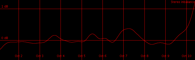 The necessary changes per
frequence bands in dB to bring the song 'in center'
The necessary changes per
frequence bands in dB to bring the song 'in center'
|
In the a-records mastering we balanced the loudness of the left and right channel automatically; and even went a step further. We measured the left/right energy-balance for each individual frequency and then brought that frequency back in balance. The above picture shows the frequency changes necessary for Rnzr track. Often the necessary changes range between -3dB and 3 dB.
Multiband compression
Another tool in the master his arsenal is the
paddle. Appropriate use of it makes the sound spank
Another tool in the masterer his arsenal is the multiband compressor. In our case we merged the compression into the above equalizer and ended up with a 4000 band compressor. The compressor had a hard wired attack/decay time of 92 msecs, but this cannot be readily perceived. Of course, it is already tricky to deal with all parameters of a 3 band compressor, set aside one with 4000 bands. To solve that we linked the threshold to a certain position in the energy histogram (e.g: at the 87th percentile) and calculated the ratio based on the maximum energy. That together with the realization that we solely work with upward compressors solved many of the parametrization issues.
Three compression curves were available. The first was an upward compressor ith a threshold at the 87-percentile energy level. The second was a saturating compressor [12]. Depending on the type of music one or the other strategy was the best. Generally we aimed to have the same dynamics across all tracks on the CD. Also here we initially relied on the ISO226 curve. That curve not only tells us how loud something should be, it also tells us how many decibels are between each 'perceived loudness change levels' (phon). Automating this process did however not work out and we resorted to manual intervention. Generally we aimed to have the maximum energy 6-12 dB away from the 87percentile energy.
One problem with multiband compressors/limiters is that they behave
differently in the transition range. As a result they are also often
used as an advanced equalization tool. In our case, we had so many
bands that it didn't really matter.
Harmonic exciting
The original 'aural' exciter has been a tool created to realign the phases of high frequencies. The reason why one needed such a tool was that in a pipeline of analogue equipment, each device would have a different, non constant groupdelay, thereby the high frequencies would loose their internal coherence. Consequently, a tool to realign the phases of these frequencies had value. However, since audiotool is all digital we don't tend to have unwanted group delays. If they are present they are part of what the artist wants to make and not introduced through the recording or so. Essentially, we no longer need to care about aligning the high frequency phases.
Nevertheless, another brand of exciter exist, which adds chebyshev harmonics to a signal. If a frequency of 4000 Hz is present, it will introduce a frequency of 8000 Hz. This type of exciter will broaden the sound and add some brightness. However, in the mastering process, we generally avoided using these because audiotool already has this type of exciter and because it modifies that what the artist wanted to make. 'If he/she wanted this thing excited he would have done that him/herself'
A third type of exciter exist, which is the 'harmonic exciter'. As opposed to chebyshev harmonics, which are type of sledge-hammer deal (you need to be very careful with the frequency transition band), an harmonic exciter will just add a slight level of distortion to specific frequencies. This type of exciter is currently not available in audiotool and produces quite brilliant results, if applied properly. When we thought some crispiness/brightness was lacking, we applied the harmonic exciter as found in izotope. Although, very few tracks improved when applying this because most of the brightness had been added through the equalizer already
Limiting
Finally, when the signal was 'ready to be burned', we need to make sure that we got as much energy as we could in the 16bits we have available. This is done by another type of compressor: a limiter.
 The band seperations used on the Flow CD
|
For the flowcd we used a self written limiter that would drastically cut out sharp peaks, and essentially remove a large chunk of the transients. This was appropriate on the flow CD, since it is all somewhat soft and easy to listen too music.
On the Affekt release, which is a more beat-oriented release, we didn't want to remove the transients. Instead there it was necessary to add body to the sound. to this end the izotope limiter was used.
Loudness leveling
Aside from making it loud, we also wanted to have all tracks equally loud on the CD. To that end we looked into loudness measurement strategies and were surprised that there are few good loudness measurement tools. In particular; the BBC has an explanation on how loudness should be measured [8]; that strategy however does not work correctly for most audiotool music because of the highly different presence of transients versus music body. Two half peak rectifiers were proposed by them to deal with this, but that didn't work for unknown reasons. Digitally, we could not reproduce the results as presented in that report. A bunch of other reports exist on how we perceive loudness, but in general little consensus exists. The strategy we finally used was to set up a amplitude histogram and match these across all tracks. That solved the problem more or less, but when listening in detail two a pair of tracks one would still hear a difference in loudness.
We didn't loudness-level the Affekt tracks.
Dithering
The final stage, was dithering: the process of fitting a continuous signal into a discrete world. When I have a sine wave with an amplitude of 0.001, then, when we digitize this signal, we can at most use 1 bit, and even that value (1) is already too large. Nevertheless that 1 bit should represent that sine wave as good as possible. That is achieved by introducing a probability that a bit is on.
When the signal is closer to the peak of the sine wave, then the probability that we output a 1, is larger than if we were at value 0 in the sine wave. This is achieved by adding Gaussian noise to the result. It improves the results of silent passages and makes the layering of multiple sounds slightly clearer. A very subtle effect nonetheless.
Conclusions
We reduced the complex process of sound equalization to about 6 parameters
- Balance between lo and hi frequencies
- Start and stop octave for the matching equalizer
- Strength of the matching equalizer
- Type of equalization target (ISO226, ITU468, K-Weighting, average CD)
- Compressor type (Plain, Knee or Saturator)
- Compressor strength
With the presented tool, the mastering round trip type has become much lower than it would ordinarily be.
Bibliography
| 1. | An Auditory Overview of some Infinite Impulse Response (IIR) Filters. Werner Van Belle Yellowcouch Signal Processing http://werner.yellowcouch.org/Papers/iirfilters/index.html |
| 2. | On the theory of Filter Amplifiers S. Butterworth Experimental Wireless and the Wireless Engineer, vol. 7, pp. 536–541, 1930 |
| 3. | Linear-phase DC Removal Filter Rick Lyons 30 March 2008; Dsp Related http://www.dsprelated.com/showarticle/58.php |
| 4. | Loudness, its definition, measurement and calculation Fletcher, H., Munson, W.A Journal of the Acoustic Society of America 5, 82-108 (1933) |
| 5. | A re-determination of the equal-loudness relations for pure tones D W Robinson et al. Br. J. Appl. Phys. 7 (1956), pp.166–181. |
| 6. | Precise and Full-range Determination of Two-dimensional Equal Loudness Contours Yôiti Suzuki, et al |
| 7. | Researches in loudness measurement Bauer, B., Torick, E IEEE Transactions on Audio and Electroacoustics, Vol. 14:3 (Sep 1966), pp.141–151. |
| 8. | The Assessment of Noise in Audio Frequency Circuits BBC Research Report EL-17 1968/8 www.bbc.co.uk/rd/pubs/reports/1968-08.pdf |
| 9. | ITU-R 468 noise weighting http://en.wikipedia.org/wiki/ITU-R_468_noise_weighting |
| 10. | Loudness Metering: ‘EBU Mode’ metering to supplement loudness normalisation in accordance with EBU R 128 EBU Tech 3341, Geneva, August 2011 |
| 11. | Algorithms to measure audio programme loudness and true-peak audio level Recommendation ITU-R BS.1770-2, March 2011 |
| 12. | A Saturating Compression Curve Werner Van Belle Yellowcouch Signal Processing; July 2012 http://werner.yellowcouch.org/Papers/saturator12/index.html |
| http://werner.yellowcouch.org/ werner@yellowcouch.org |  |