| Home | Papers | Reports | Projects | Code Fragments | Dissertations | Presentations | Posters | Proposals | Lectures given | Course notes |
|
|
Training a Distance MetricWerner Van Belle1 - werner@yellowcouch.org, werner.van.belle@gmail.com Abstract : This article explains how to train a distance metric in a multi-dimensional space.
Keywords:
distance metric learning, weighted metric |
Table Of Contents
Introduction
Given a multidimensional space containing points, with each point being a feature vector. Each vector contains multiple values, each representing a property of an underlying object. In case the feature vectors represent songs, the first dimensions could reflect equalization information about the song. Other dimensions would contain information on rhythm or loudness characteristics. Given such a series of vectors, the natural question to ask is how we can compare them in such a way that the comparison makes sense to humans. It is after all not to be expected that humans would treat all dimensions as equally important. Equalization might be, or not be, more important than the loudness characteristic of a song.
In order to create a distance metric that reflects the human perception sufficiently close, we created a distance training algorithm. The distance metric being learned is a true distance metric, in the sense that it will never produce negative values, and it is trained on a series of 3 way comparisons between points.
The data set
Although the algorithm does not depend on the dataset, it might be useful to work with a concrete example. As could be gathered by now, we are talking about songs in a multi dimensional space. Each song is represented as a point in this space. The features are extracted using various algorithms, including tempo detection [1, 2, 3], rhythm pattern extraction [4], loudness information extraction and equalization information. The description of the various dimensions is given below.
- Dimension 1: length of a measure (which is the tempo)
- Dimension 2 - 385: rhythm pattern for the lo frequencies, 2 bars, 192 ticks per bar.
- Dimension 386 - 769: rhythm pattern for the middle frequencies, 2 bars, 192 ticks per bar.
- Dimension 770 - 1153: rhythm pattern for the hi frequencies, 2 bars, 192 ticks per bar.
- Dimension 1154 - 1164: loudness information for mp3 subband 0. 11 values, reflecting the energy value at quantiles 0 to (including) 100
- Dimension 1165 - 1483: loudness information for mp3 subbands 1 to 29.
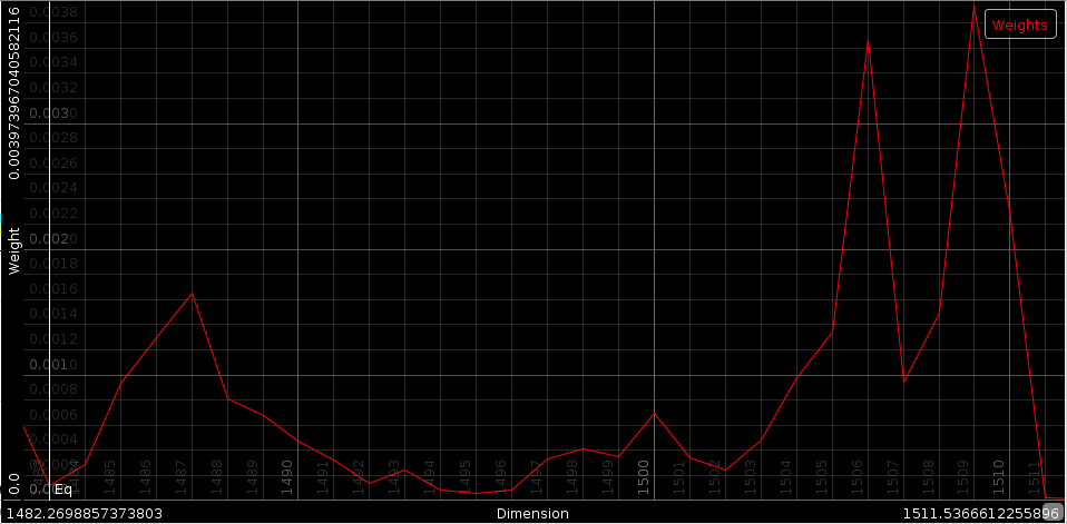
- Dimension 1484 - 1513: equalization information for mp3 subband 0 to 29 of the mp3.
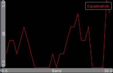
The principal distance between values for the tempo is the distance between their log values. The distance between the rhythm patterns is given as the sum of the absolute difference between the energies, after normalizing each band by subtracting its average value. The distance between loudness bands is calculated by matching each loudness band to a target profile, which is the average loudness as found in the whole data set, and then calculating the sum of the absolute differences. The equalization parameters are compared in a similar manner. Each equalization profile (all 30 values), are first converted to dB, then brought to a mean value of 0, after which their absolute differences are summed together.
| ||||||
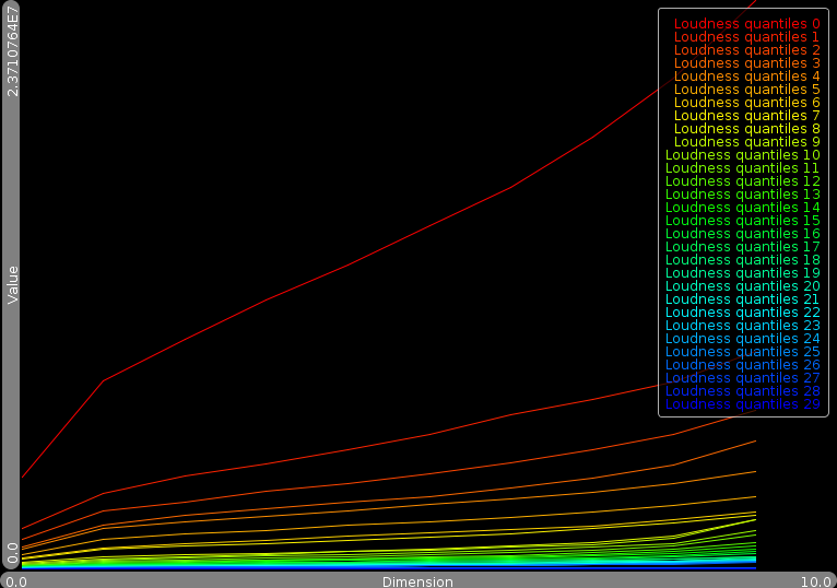
| The Rhythm property is shown as a two dimension image. Horizontal the position in a bar is set out. Vertically the frequency. The intensity of a pixel is the value at that position in the bar/frequency domain. The eq property are 30 values, reflecting 30 subbands of the mp3 data. Expressed in dB. The loudness property are the decile quantile values for the 30 subbands we measured. |

Obtaining information from the user
To obtain information on which features are important to the user, we started out by presenting him/her with a series of 3-point comparisons. We would present him/her with 3 songs (A, B and C) and ask him whether B or C was closer to A. Of course, after a short while, it became clear that this was a very tedious process and we could obtain relative more information by presenting him/her with more songs. So we ended up with a sixteen song test.
The sixteen song test presents the user with a target song and 15 songs that he/she has to group in near/far songs. If a song was broken, impossible to rate or other problems occurred, it could also be omitted from the grouping. A sixteen song test is saved as
A target song
A list of winners
A list of losers
The advantage of using this more difficult test is that we get more data from each presented song. After all we can compare eachof the winners against each of the losers
foreach(test:16songtests)
  foreach(winner:test.winners)
    foreach(loser:test.losers)
      generate-tripler(test.target,winner,loser)
In other words, we always end up with a set of triplets, specifying the target, the closest song and then the furthest song.
Statistical Generalisation
Using this data we could try to train a set of weights directly such that the resulting distance metric would produces the correct tuples in as many cases as possible. (we write subscript c because this is the computer generated distance metric. Eventually we will need to make a distinction with the distance information provided by the human, in which case we use h as a subscript.)
The problem with this approach is twofold.
Overfitting. The first problem is overfitting. Given 1513 dimensions, and let's say 44'000 distance comparisons. The chances that the algorithm will always find some dimensions it can use or abuse to get a triplet matching is fairly high. That is to say, the algorithm might select a noise feature (one that we really don't care about), and use its values across the 44'000 comparisons to get two or three triplets correct. After all it has 1512 dimensions left to deal with the other problems.
Irrelevant model. A second problem is that let's say, 1000 test have been performed, generating on average 44 triplets, which results in 44'000 distance comparisons. From all the songs we have we can only look at the comparisons that were presented to the user. If the algorithm were to take songs X,Y and Z and no comparison (X,Y,Z) or (X,Z,Y) was generated during training, then the algorithm will have no idea how to update the weights. Essentially, from a total set of 300'000 songs, such test set would be a mere 9.7E-5 percent of the whole dataset, or stated differently, we would be omitting 99.999902 of the full potential for testing we have.
|
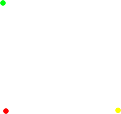
To solve these two problems, we generalized the results and counted how many times the distance for each dimension was reporting the same as the overall distance. The above image illustrates how this works. Suppose we asked the user whether the yellow or the green dot was closer to the red, and suppose that he answered yellow. In that case we know that the horizontal axis is more important for him than the vertical axis. Likewise, if he would have answered the green dot, then we would know that the vertical axis carries more weight. By counting how often the horizontal axis reported the same result as the overall distance, we know indirectly how important that axis is.
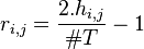
Formally, based on the set of triplets, we can calculate how often a specific feature is in alignment with the actual measure. T is our test set of triplets and d is the human distance metric:

The set of points where dimension i suggests the same as the overall distance measure is defined as

To convert this to a number that specifies how often dimension i aligns with the end result, we calculate
h_i is 0 when that dimension absolutely always fails to reflect the end result. That means, that if dimension i is close, that the final result will likely be the opposite. In the same way, if h_i is 1 then dimension i very consistently predicts what the end result will be. Generally the values will center around 50%
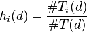
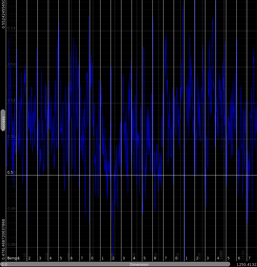
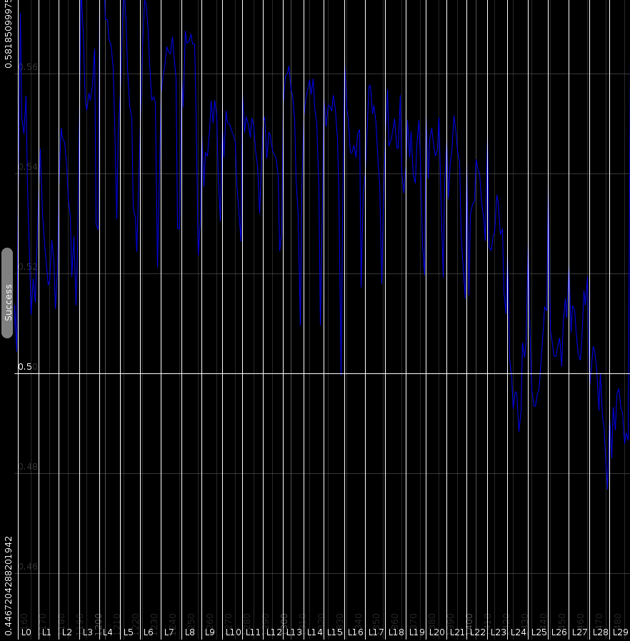
| ||||||
| Plots showing how often the distance along one dimensionwould report the same as the overall perceived distance. Horizontal the various dimnesions are set out. Vertical, the relative count (h_i) |
Standard learning algorithms
With such statistic in hand, one could consider using them directly as sort of weights. That does however not work because it is merely an interpretation of the information given to us by the user. They are not direct weights. Instead. the method we will use is to generate a distance metric that produces similar statistics as the ones we just obtained. With each step we will
- generate the statistics
 using the
alignment counts when using the learned distance metric:
using the
alignment counts when using the learned distance metric:

- for each dimension compare
 against
and adapt the weights
against
and adapt the weights 
- repeat until satisfaction
In the above, d_h is the distance metric as obtained from the human
through testing, and although we don't have a evaluable function
for it, is still known.
Initially we used Q-learning to train the weights, but never got it working completely right. Often certain weights would keep on increasing, and no matter how much the algorithm increased them, it could not match the required statistics. At other dimensions, the opposite happened. Weights kept decreasing. It even drove us to the point where we would allow negative weights and started to train a distance function instead. However, we did not feel particularly happy about such approach because it makes no sense to have negative distances between songs.
After studying the problem for a while we figured that the problem was that many dimensions acted in group. That is to say, if beat 1,2,3,4 all correlated positively towards the distance metric, then some algorithms would tend to focus only on, let's say, beat 3, and lower the weights of beat 1, 2 and 4. After all, beat 3 contained largely the same information as beat 1, 2 and 4. However, it felt wrong, because in those instances that beat 3 actually mattered, the metric would be blind to it. It did however reveal the problem: the internal structure of the space. The dependencies between the various dimensions would lead to weight adaptations that would work against each other, pushing the problem around until some irrelevant dimension would aggregate the garbage.
To solve this we set out to explicitly take into account the dependencies.
Internal Structure
We calculate the dependencies between dimensions by counting how often the distance on dimension i aligns with the distance on dimension j. The dependency matrix:

h_i,j describes how often dimensions i is in alignment with dimension j. Based on that we can define a sort of correlation value by normalizing it to fall within -1:1
 A demo of the correlations between dimension 82 (where the red spike is) and all other dimensions. The red line shows h_i,j, with i=82. Horizontally, two bars of the low frequency of the rhyhtm patterns is set out. Vertically, the correlation strength.
|
Training using the dependency matrix
With such a correlation matrix in hand it is much easier to calculate weights such that d_c matches d_h as close as possible. In the equations below we write  , that is h_i are the statistics as obtained from the test set, while
  are the statistics as obtained from the trained distance metric.
Updating the weights happens as follows
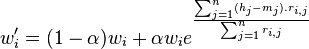
A number of observations led to the above equation
- when working with large dimensional spaces distances behave logarithmically. The larger the space, the more distances will be all more or less the same. By modifying the weights exponentially we have the tool to actually create an effect. Linear modifications almost never cut it
- The weight of dimension i is modified by integrating all the wanted modifications on all other dimensions and how their wishes (h_j-m_j) translate back to our dimension i.
- The overall modification is of course related to how much change we can expect from the various dependencies, so we normalize it by means of the denominator
- Alpha reflects the learning rate. It should start with 1 and slowly decay. As time progresses less and less change is allowed to the weight vector.
Weights
Using the above algorithm on a test set of songs from BpmDj, we obtained the following weights for the importance of the various dimensions.
| ||||||
| The compiled weights |
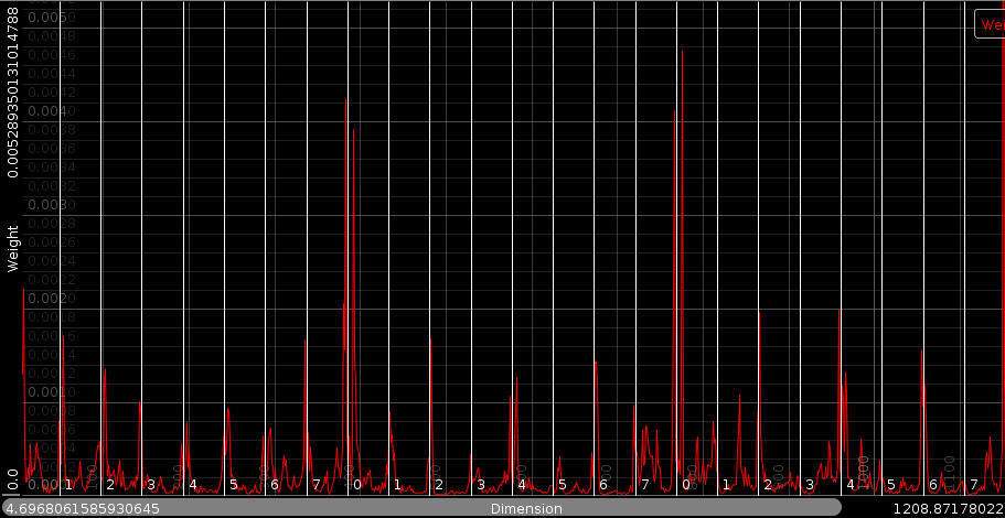
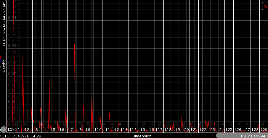
Rhythm weights - important positions are the beginning of each bar. (The lo middle and high frequencies position 0 have a high weight). The relative weight ratio between lo and hi can be explained by the fact that the hi frequencies have generally a lower amplitude, resulting in a strong weight requirement for them. Of course, the beat between two bars (the fourth beat in a two bar rhythm) is important, but only in the high and middle frequencies. Another interesting observation is that important rhythm factors are always a bit behind or in front of the position of a beat, they do not literally fall on the beat. That could be explained by the onset and drag a sound has. We apparently find that important.
Equalization weights - the important positions peaks in the equalization weight diagram are at band 4, 23 and band 26. These correspond to frequencies 2756Hz, 15000Hz and 18000Hz. Not much unexpected.
Loudness weights - The loudness weights have almost all an important 8 decile but almost no others. This is a bit unexpected and might lead to new loudness measurement modules.
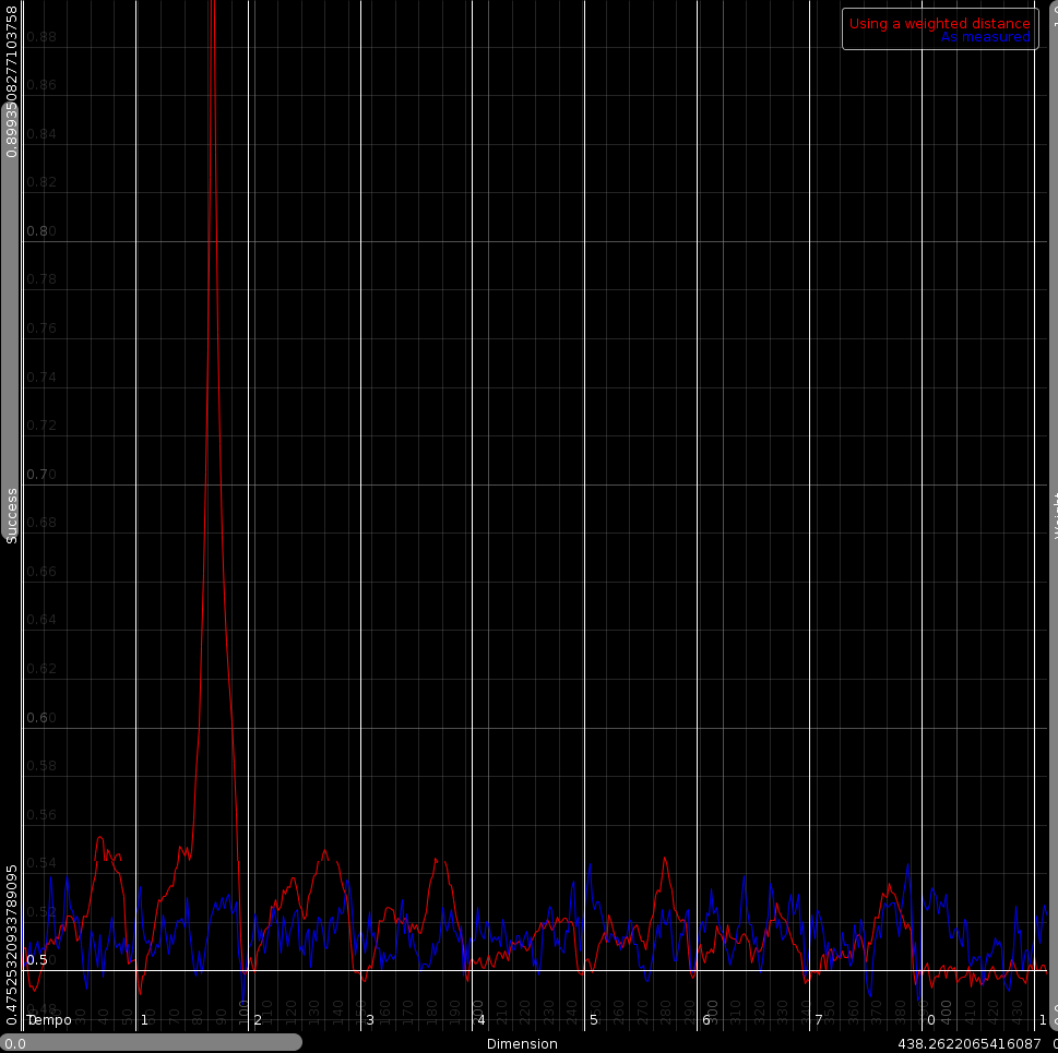
Using these weights, we can check whether the weighted metric behaves similarly to the human metric.
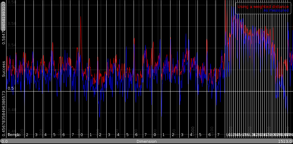 The statistics using the weights. The red line is the weighted metric. The blue line is are the statistics obtained from the testset.
|
Conclusion
We presented a distance metric learning algorithm. It 1) uses triplets from a test set containing near and far information. 2) It then generalizes these into a general purpose statistic, describing which dimensions align with the overall metric. 3) To deal with the problem of dimension groups, the internal structure of the search space is determined by analyzing dependencies between dimensions. 4) That information is then used to train a weighted metric such that the statistics of the metric match those of the human test set.
The result is a quickly converging algorithm that can generate anti-correlation without resorting to negative weights.
Bibliography
| 1. | Fast Tempo Measurement: a 6000x sped-up autodifferencer Werner Van Belle Signal Processing; YellowCouch; July 2011 http://werner.yellowcouch.org/Papers/fastbpm/ |
| 2. | BPM Measurement of Digital Audio by Means of Beat Graphs & Ray Shooting Werner Van Belle December 2000 http://werner.yellowcouch.org/Papers/bpm04/ |
| 3. | Biasremoval from BPM Counters and an argument for the use of Measures per Minute instead of Beats per Minute Van Belle Werner Signal Processing; YellowCouch; July 2010 http://werner.yellowcouch.org/Papers/bpm10/ |
| 4. | Rhythmical Pattern Extraction Werner Van Belle Signal Processing; YellowCouch; August 2010 http://werner.yellowcouch.org/Papers/rhythmex/ |
| http://werner.yellowcouch.org/ werner@yellowcouch.org |  |