| Home | Papers | Reports | Projects | Code Fragments | Dissertations | Presentations | Posters | Proposals | Lectures given | Course notes |
|
|
FlowPipes: Isolating and Rejoining Data Tokens in the context of Data Analysis PipelinesWerner Van Belle1,2 - werner@yellowcouch.org, werner.van.belle@gmail.com Abstract : FlowPipes is a data processing abstraction that helps to integrate data analysis modules into a data analysis pipeline. The infrastructure provides automatic joining of relevant data as well as rejoining of the analysis output into the overall flow. FlowPipes explicitely separates a meta-level (in which tokens drive the computation) from an object-level (where commands process raw data). The computation is driven through tokenmatching: when data-tokens can be combined then the computation continues along that path. The resulting pipelines are data-driven and programatorically functionially oriented. We demonstrate our work on two bioinformatics examples: a real time PCR calculator and an image correlation tool.
Keywords:
bioinformatics analysis pieline, flowpipes, 2d gel correlation, rtpcr, qpcr, realtime pcr, quantiative, petri-nets, functional, guards, places, transition, tokens |
1. Introduction
FlowPipes was born from the common problem to integrate a fairly simple and modular algorithm into a real life workflow. Often one spends 50% time on creating an algorithm and debugging and testing it and then another 50% to make it run through an actual dataset.
An actual dataset often poses problems because they tend to have different internal groups (E.g: patient A in condition B against patient C in any possible condition) and the same algorithm needs to be ran on different groups. Whenever a new dataset comes in it is not uncommon to be faced with a new group structure. Surprisingly enough without a proper support infrastructure, this type of 'small' changes tends to be quite costly for the developers. Sadly enough, partners (especially if they are biologists) often have problems grasping the complexities of data grouping and data integration in many cases. As such we set out to find a good strategy (and architecture) to deal with this.
To our surprise we didn't find many good abstraction to deal with this challenge. Of course, the most basic abstraction is that of a pipeline: we have certain modules which process data and then pipes which deliver data from one module to the next. This simple idea is very powerful and omnipresent in the field of bioinformatics. Regardless of this existing idea, proper computational abstractions to describe such pipeline are hard to come by, especially if one start to think about real life requirements:
1. flexible - we want the ability to change the pipeline such that the resulting modifications are as one would expect, while not loosing the old processed data. That is to say: suppose we want to add an extra element to the data: e.g: a name of a person. Then we expect this information to be automatically being propagated throughout all accessible pathes in the pipeline.
2. efficient - we do not want to compute the same thing twice. A change in one of the modules of our pipeline should not trigger a full recalculation.
3. persistent - the obtained/calculated results should be stored such that we can easily access them, without the potential of accicendataly seeing them deleted through a cascading effect in the beginning of the pipeline.
4. distributed - data processing in bioinformatics is sometimes computationally challenging. As such, one might need to place multiple modules at remote machines.
5. no concurrency problems - face it: concurrency problems are here (and there and there :-)); but when you work with data you really don't want to think about them. You want things to flow smoothly without having the typical problem of interacting processes: deadlocks, corrupted data and so on.
To satisfy these requirements, we experimented with a number of different models. Some of them were incapable of even expressing the most basic problem, others were so general that we were actually programming our pipeline each time. The most usable abstraction was that of Petri-nets, however it had to be modified substantially to become usable (see later).
From our point of view FlowPipes satisfies all the above requirements while still being fairly orthogonal and sufficiently dense, so that the description of the operational semantics would not take too much space.
2. Cases
We now discuss two examples with which we will work later on
1. Image correlations across parameters and patients. This example shows how the FlowPipes joining operation eases the development process. One mainly needs to focus on the correlator routine itself. The extra meta data, such as patients information, can easily be used to group the dataset in different manners.
2. Quantitative PCR calculations. In this example we have a number of plates, on each plate we have a number of positions which belong to the reference gene or measured gene as well as positions that belong to the wildtype cells against the transgenic cells. Each measurement can have multiple replicas at different dilutions. These many intertwined groups needs to be properly selected and regrouped before an analysis can be conducted.
We explain each of these examples in more detail
2.1. The P53 Image Analysis example
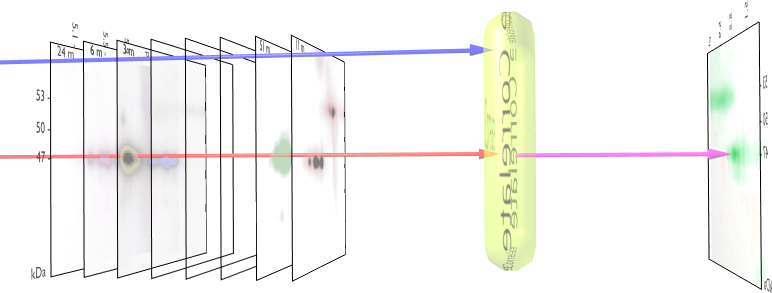
Figure 1. Correlation Overview
This is the first example we got involved with in 2004. It is about the analysis of 2DE gels against a number of biological parameters. The algorithm core is a simple lineair pearson correlation, but modified to work on images. It takes a number of images, each tagged with a number and then correlates each pixel against this colledion of numbers. It reports on the areas in the image had the highest correlation against this external vector. In particular this led to new insights between P53 and cancer. See [1, 2] for a detailed description of the method. An example analysis can be found in [3, 4]. Figure 1 illustrates the process.
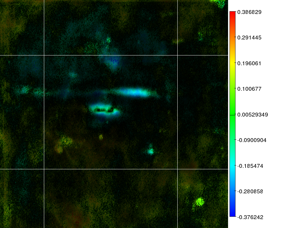
Figure 2. P53 correlation demonstration. The color in the image reflects the correlation strength as given in the heatbar to the right. The darkness/brightness of each pixel reflects the significance of the correlation.
Figure 2 demonstrates the output of a correlation analysis between P53 isoforms and the AML FAB classification. It reports which areas of the 2D gels would not relate at all to the FAB classification, and which ones would. Both pieces of information are very valuable. Aside from the correlation image, the algorithm would also generate a significance map to show which correlations were very likely to be random occurrences and a mask image which would only keep those areas on the map where there was at least something base some form of prediction on. (That is to say: certain areas could produce a correlation, but without much signal variance in the images; essentially making the correlation useless)
Now, the above algorithm is simple. It takes 2 inputs and produces 3 outputs. The first input is a collection of images. The second input is a collection of numbers (one for each image). The first, second and third outputs are respectively the correlation image, the significance images and the variance image.
When working with the full sized dataset we found that the integration of this algorithm into a pipeline caused some headaches, mainly due to the sheer amount of group-types involved. We received data for 2 diseases (AML and ALL) of around 100 patients. Most patients had 0, 1, 2 or more 2D gels made. These gels were grouped into timeslots (when were they made), by whom they were made and which technique was used to obtain the image. As such we had a group of old gels which were X-rayed to detect protein presence (XRay), we had 'old' gels which were stained using a differente procedure (Old). Afterward a number of these gels were redone twice, resulting in replicas for most of the patients: we call these two extra runs: (Gel1) and (Gel2). A third variable were the different biological parameters for each patient, totalling another 137 variables. Of course, the various combinations between boligical parameter and gelimage group did not always produce an overlap. It was for instance often the case that a certain patient might not have the required image, nor might (s)he have a value for the required biological parameter.
Based on these multiple inputs we had to streamline all data so that we could at least get it into our pipeline. This involves checking whether a numerical variable only contains numbers and not strings such as (>10, <12) Afterwards, we had to create all potential combinations so that the biologist could explore the various datasets. However, since the biologists did not know which type of gel image they wanted to include in the analysis we had to create groups of gels. E.g: the new gels could have been of better quality than the old. Then we shouldn't include the old. Or the XRay only gels might have a better information acquisition; so then we should not mix them with others etc. In the end we created 8 groups of gel images:
1. Gel1: is an image set containing the first batch of gels
2. Gel2: is an image set containing the second batch of gels
3. Gel1&2: is the union of group Gel1 and Gel2
4. Old: are all the initial images, excluding the X-ray images.
5. XRay: are all the X-ray images
6. AllWithoutFilms: is an image set containing Gel1&2 and the Old collection, excluding the X-ray images.
7. AllWithFilms: is an image set containing all Gel1&2, Old and Xray.
8. OldWithFilms: is an image set containing only the Old dataset, including the XRay images.
The biological parameters were the following genes, variables and other properties: CCL1, CCL13, CCL17, CCL2, CCL20, CCL22, CCL23, CCL24, CCL26, CCL28, CCL3, CCL4, CCL5, CCL7, IL1b-0, IL1b-CXCL10, IL1b-CXCL11, IL1b-CXCL4, IL1b-CXCL9, IL8-0, IL8-CXCL10, IL8-CXCL11, IL8-CXCL4, IL8-CXCL9, age, basalphosphor, bcl2, cd11cbis, cd13bis, cd13num, cd13yn, cd14bis, cd14num, cd14yn, cd15bis, cd15num, cd15yn, cd33bis, cd33num, cd33yn, cd34bis, cd34num, cd34yn, clustergroup, cytobad, cytoclass, cytokineresponse, delnp53, dnp63, erkconst, erkflt3l, erkgcsf, erkgmcsf, erkifng, erkil3, fabm, flt3itd, flt3lmnum, flt3lmwithoutwt, flt3mut, flt3riskgroup, flt3seq, flt3seqgroup, fltasp835num, hb, hclgroup, integratedbiosig, jonathan2dratio, karyotype, karyotype2, lpk, nina2dclass, npm1, numflt3itds, p38const, p38flt3l, p38gcsf, p38gmcsf, p38ifng, p38il3, p53, p53b, p53g, p53stat, p63alfa, p63beta, pbest3, prevdis, ptotal, relapse, resistance, resistc1, ser15, ser20, ser37, ser392, ser46, sex, stat1const, stat1flt3l, stat1gcsf, stat1gmcsf, stat1ifng, stat1il3, stat3const, stat3flt3l, stat3gcsf, stat3gmcsf, stat3ifng, stat3il3, stat5const, stat5flt3l, stat5gcsf, stat5gmcsf, stat5ifng, stat5il3, stat6const, stat6flt3l, stat6gcsf, stat6gmcsf, stat6ifng, stat6il3, strictsurvival, strictsurvivalwithout0, survival, tap63, tpk, wbc. Clearly a long list and it would takes us too far of track to explain any of these variables.
A last consideration was the fact that we could or could not normalize each image before it went into the correlator. Since we didn't (and still don't) know whether the images should be normalized or not; it made sense to also include this type of analysis.
In summary, the data structure for this problem can best be described by a number of statements
1. each patient has multiple gel images
2. each gel image belongs to one or more image group (one of the above 8)
3. each patient might have a value for a specific biological variable (one of the 137)
4. gel image can or cannot be normalized
From all the numbers above we quickly come to a staggering amount of analysis to be done. With 8 image sets, 2 normalization schemes, 137 parameters we had to generate around 2192 correlation images and report them back in a somewhat sensible manner. Of course this number is somewhat exaggerated since we did not always have a sensible correlation map due to too few data points (in either the image collection or the biological parameter collection); but this again added to the challenge. It was not only a matter of computing one group against the other; we first had figure out which data point actually appeared in both sets (that is the image set and the biological parameter set).
At first sight this is a simple matter of combining the datasets in a procedural manner and compute the results
  foreach parameter do
    foreach imageset do
      foreach normalization do
        SELECT images, value
        FROM Patients, Images, Parameters
        WHERE ...
However, given the time it takes to generate a correlation map (and associated movie), we needed 8 machines to compute this to be able to finish it in a couple of months. So we were looking at an extra non functional requirements: a distribution problem. Another problem with this scripted SQL approach was that of incremental data addition. What happens if a new image comes in or when a new parameter of a patient becomes known. Which correlation maps are affected by that ? This was also important since we did not want to recompute the elements that were not affected. So we needed something which was smarter than an ordinary join on two or three database tables. It had to remember which combinations were already calculated and what the results were (caching).
One might now think that makefiles might work, but the reality is that makefiles are not so very good at creating all these different combinations of database tables. Makefiles were also not very good at dealing with the distributed processing of data. One might consider generating the makefiles but then one is again solving the original problem of generating the proper combinations. One particular paper that appeared at that time was on makefiles using horn-clauses where the makefile groups were actual makefile targets as well. This made it possible to parametrize the makefiles much more natural than what can ordinarily be done. However, the lack of distribution and the rule based approach still forced us to think about quite a lot of non-functional requirements [5]
2.2. qPCR Analysis
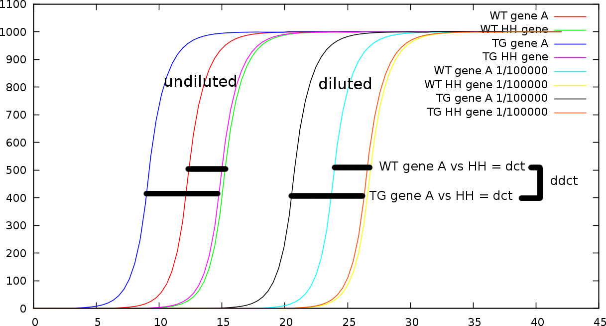
Figure 3. qPCR overview.
The second example we investigate is a quantitative PCR analysis.
qPCR is a technique where one uses two types of cells, for instance
wildtype (wt) cells against transgenic (tg) cells. For each celltype
one measures two genes: a gene which is considered to be the household
gene, and expected to have the same expression in both cell lines, and
the gene of interest. So this leads to four measurements. Of course one
performs a number of replicates leading to 3 measurements for each of
the 4 genes. Once these values are obtained the differences between the
gene of interest and the household gene are calculated and then
compared across the cell types. This lead to a report on the up- or
down regulation of the gene of interest. Figure 3 illustrates the various possible
measurements. Horizontally the graph show the number of cycles
necessary to reach a certain amount of material (which is set out
vertically). Based on the number of cycles one can estimate the
original concentration. Figure 3
contains both a strongly dilluted (1/100000) measurement and a normal
measurement. What is first calculated is the  -value between the gene of interest (in this case A) and the household
gene. This value is the difference in number of cycles necessary to
reach the same volume. Once the two
-values are known one can compare the relative expression of gene A
between the wildtypes (WT) and transgenic (TG) cells; which gives the
-value between the gene of interest (in this case A) and the household
gene. This value is the difference in number of cycles necessary to
reach the same volume. Once the two
-values are known one can compare the relative expression of gene A
between the wildtypes (WT) and transgenic (TG) cells; which gives the  -value.
Of course, there are some complications with this method. Since it relies on a specific number of amplification cycles there is a sensitivity issue. If we require too many cycles to have a proper measurable amount, we cannot accurately obtain the initial concentration. If there are not sufficient cycles we cannot estimate the efficiency. So one needs to wait the proper amount of cycles. However, if the exponential process reached its limit (a well can only contain so much biological material) the measurement also becomes problematic. To tune this one relies on a number of dilution series such that the number of cycles between the household gene and the gene of interest fall nicely within a 10 to 30 cycle window. So for each of the measurements we also have a number of dilutions such as 1/1, 1/5, 1/20, 1/50.
Now this small addition makes the calculations difficult because the dilution series tend not to affect the difference between the household gene and the gene of interest, it does however affect differences between the genes across dilution series. So in other words, one cannot first average out all genes independent of the dilution series, one can however take the average of the difference between the gene of interest and the household gene. Figure 3 illustrates this. The lengths of the bars in each dillution serie is the same.
3. FlowPipes Overview
3.1. Functional style
To deal with the above cases, where we have a core algorithm (termed analysis module) wrapped in a practical dataset/pipeline, we created a form of super-processor that would take care of analyzing the required combinations and executing them. As potential abstraction to create this super-processor, we first looked at Petri-nets [6, 7, 8], which turned out to be very modular, which was a good thing, but they also make expressing simple things difficult. One of the most elegant features of Petri-nets is that they are very efficient in modeling concurrent systems, however that was a bit of a disadvantage because very often we had to write contorted construction to inhibit concurrency. We found that we spend more time managing concurrency problems within a Petri-net than actually caring about the composition of the different modules.
A second problem of Petri-nets was that it was fairly complicated to distribute analysis modules automatically ovcer multiople machines. That is to say: either tokens were self contained, in which case we had to understand the data format completely (see later), or tokens were not isolated, in which case transporting a token to a client machine could cause problems. E.g: suppose we have a token stating that a specific file in a folder on a particular machine has the image. If we transfer only this token to a client machine, then it is not at all clear whether this client machine will be able to retrieve the other piece of data. It is of course not difficult to add some annotation that would be able to copy this file but then very quickly we end up in major concurrency problems, unless we create new data and never modify existing data. At this point we realized that a functional approach was the only sensible way forward. As such we tried to modify the Petri-nets abstraction in a functional manner.
3.2. No seperation between metalevel data and objectlevel data
A major problem always came about when we tried to separate the meta-level (the tokens that drive the computation) from the object-data (the data used by the commands; E.g: raw images.
Consider this example: assume we have a collection of images, that, as already described, can be put into a correlator module. In this case the iamges would be considered the object-data since the correlator module would access them. The metadata, such as to which datagroup they belong, would be considered metadata. Assune now that the requirement was to analyze all images that have a size smaller than 1000 pixels. This is typically a meta-level question because the selection of images needs to be decided at the meta-level. This makes the imagesize a metalevel piece of information. However, the correlator clearly cannot work without knowing the imagesize. So we have a transgression between levels.
Whatever way we looked at it, we found no possibility to sepearte the metalevel from the objectlevel without requiring too much knowledge of data formats. Our data architecture would essentially require full knowledge of all the object structure passing through it. We did not want that. The architecture should only require the pieces of information it needs at that particular level.
3.3. Data Tokens
Because we try to modify the Petri-net abstraction to deal with data in a functional manner, it becomes time to think about the data tokens that will pass through our net, and consequently what grammer would be used to describe guards and input/output expressions of the transitions.
One very quickly thinks of hierarchies of data: e.g: a filesystem hierarchy, a token would then be a pathname. Hierarchies seem attractive because one can nest tokens into one another, but that approach led us nowhere. We ended up in contorted manners to find data in such trees. Similar problems exist in object oriented databases. And although data normalization schemes might be a way forward, they would beat the purpose of making our system 'easy to use'.
After a while we realized it made more sense to fall back to the remarkable efficient and simple setup of relational database. A token would then be output from such a table.
3.4. Places
The transmission of information happens at two overlapping levels. The metalevel deals with deciding which calculations should take place. This information belongs to the 'pipes'. The objectlevel contains the content of the various tokens: these are files on disk etc. All tokens are transferred from one place to the next. A place itself is a table, containing attributes (of a specific type) and fields, very much like a table in a relational database. The advantage of using this approach is that it is easy to convert such a table to a tab separated file that is passed along to various commands and the output of a command can also easily be read in again in this type of tables.
For instance in our P53 example a place would store the location of the images for each of the patients. This would be described as (patient, image). The content of such a place could be for instance
  patient  image
  WVB      nicegel1
  WVB      nicegel2
  WVB      gel-XR
  KTY      badgel1
  KTY      kty-gel2
As can be seen in this case each patient is associated with multiple images, each image representing a replica experiment.
Another example of a table could be to describe to which group each gel belongs. This (image, gelgroup) place can have content as follows
  image     gelgroup
  nicegel1  New1
  nicegel2  New2
  gel-XR    XR
  badgel1   New1
  kty-gel2  New2
One database table is one place. Depending on how data is extracted we can have differente tokens in the same table.
3.5. Grouping
Because each place must be able to contain multiple tokens and because each token is a tab seperated file, we had to think about annotating the elements of the table to describe to which token they belong. We could add an extra attribute to the table/token to annotate to which token a particular row belongs. That however was problematic since often the interpretation of what constitutes a token can change. For instance in the P53 example we might want to retrieve one token containing all (patient,image) information, however in another situation we might choose to retrieve all image information for a patient.
To solve this we introduced the concept of data grouping, which is annotated with a *. To express this in normal relational database terms: every attribute that is not grouped belongs to the primary key.
Suppose we have the place (alfa,beta) with the elements
 1  test
 1  pest
 2  test
 2  pest
then the multiple tokens would be the subtables
 token 1: 1 test
 token 2: 1 pest
 token 3: 2 test
 token 4: 2 pest
If the table were defined as (alfa,beta*) then the tokens would be extracted solely on the alfa attribute; and thus result in:
  token 1:
    1 test
    1 pest
  token 2:
    2 test
    2 pest
If the table were defines as (alfa*, beta*) then the only token present would be the place itself
 token 1:
   1  test
   1  pest
   2  test
   2  pest
3.6. Commands
A command is a process which takes a fixed number of inputs, each of them tab separated files, and produces a fixed number of outputs, each of them tab separated files as well. Together with the tab separated files which contains the meta-data, the data which the command should be dealing with can be stored somewhere in a directory. Important is that no command shall modify any of the input data. As such if new files are to be created then they should have a well laid out target destination.
For instance, in the P53 example one of the commands would take a stack of images together with a biological parameter and generate a new output image (the correlation map). In this particular command there is only one input: a csv file of format (image, parameter). The image being the filename of the image on disk and the parameter being a number. The image of course must exist somewhere on the file system and is also part of the command input. The output of this command will be an (correlation, significance, mask, count) CVS table, which will contain only one row. Correlation will refer to the correlation image, significance to the significance calculations, mask to the variance mask and count is a number reflecting how many images were actually used in the calculation. The three generated images must be dumped somewhere on the filesystem and once they are dumped they should not be lightly relocated.
3.7. Transitions: weaving commands together
The commands describe the external analysis modules, with strict defined and generally usable inputs. Of course, these commands needs to be placed in the overall layout of the data flow. This is were transitions come into play.
Each transition acts as a wrapper around a command. A transition is responsible for
1. retrieving the tokens to be passed into the command
2. executing one or more commands in parallel: if we have an external command that will work on a file list associated with a specific patient and produce one output file, then the input into this command is a (patient,file*) group while the output will be a single row of (patient,file) data. Now, since we know the grouping the flow execution can call multiple commands at once, each having its own file collection per patient.
3. retrieving the output of each command and merging it back into the pipeline. This is the most important work of a transition. It allows commands to work only with the data they are interested in. E.g: we could have a command that converts a collection of images into a movie. Of course this movie will indirectly belong to a patient-biological parameter combination. However, that information: which patient and name of the biological parameter is strictly speaking not necessary to create the movie. As such; the transition will first extract the relevant information (only the generated images), pass it to the command, which will generate the movie and then rejoin it with the patient and biological parameters which were involved. We will describe the operations necessary for this conduct somewhat later on.
4. observing the potential combinations of inputs and selecting those that make sense in the data flow.
5. ensuring that no unnecessary calculations take place (caching)
6. deciding what to execute when a particular output is required
3.8. Selecting Attributes
Each transition takes input from a fixed number of input places, has a command associated with it, and produces output for a fixed number of output places. The input and output places are ordered in accordance with the inputs and the outputs of the command. If more inputs are necessary to drive the computation or limit the possible combinations, but of which the input is not used by the underlying command, then these should be placed after the standard inputs. A transition might look somewhat like
  Correlator(Input(images,"image","value"),
             Output(result,"correlationmap","significance","mask","count"))
In this case the command is the 'Correlator'. The first input are the images and only the image and value attribute are passed along. All other attributes that might be available in the images place are not passed into the command. The output of the command, which as described before will generate 3 images and a count, are placed into the output place 'result'. Each column of the output file is dumped into the respective attributes.
In this example, the tokens passed into the correlator are dependent on the grouping of the images place. The transition will simply iterate over each of the tokens present there and for each token call the command.
As an example: if we have an images place of type (image*, value*, dataset) with the following data
  image  value  dataset
  A      1      alfa
  B      2      alfa
  C      3      alfa
  D      1      beta
  E      2      beta
  F      3      beta
then we will pass only two tokens into the correlator: the alfa and beta dataset. However, the dataset attribute is not passed into the command either. What the Correlator will see are:
  A  1
  B  2
  C  3
and in a second call to the command
  D  1
  E  2
  F  3
In both cases will the command generate a new output which will be placed into the results place. The two output tables could be
x1 y1 z1 c1 (for the alfa dataset)
and
x2 y2 z2 c2 (for the beta dataset)
with x1, y1, z1 and c1 the correlation image, standard variance image, mask image and correlation value.
3.9. How a transition integrates a commands' output
If the output of the above example were instead defined as (correlation, significance, mask, count, dataset) then the original dataset attribute would behind the commands' back be passed along as well: resulting in a results table
  x1 y1 z1 c1 alfa
  x2 y2 z2 c2 beta
This is where the full power of our FlowPipes can be demonstrates. The commands are modular since they do not need to care about extra contextual data and the transitions have very sensible defaults to pass extra input parameters to the output as well, such that only compatible data is combined (with the same attributes on anything else that is not passed into the command).
If we now look back at our example and assume that the inputs have a different grouping strategy. Suppose the images place was declared as (image*, value*, dataset*). In this case there would be only one token present at the input and the correlator would be called on the entire dataset
  A      1
  B      2
  C      3
  D      1
  E      2
  F      3
resulting in an output of
x3 y3 z3 c3
Because the dataset attribute was grouped in the input it will not be rejoined in the output and it is actually lost. The reason behind this is that the grouped attribute in this case would produce too much output if we were to rejoin them. Although in this case we might image the generation of
  x3 y3 z3 c3 alfa
  x3 y3 z3 c3 beta
It is difficult to imagine what we need to generate if the correlator command would produce an output with 100 rows. Then we would need to take each row and generate the alfa and beta variant. Clearly this type of data size explosion is unwanted and will clog the flow system very quickly.
3.10. Joining of inputs
Because commands can take multiple inputs it is necessary to define which combinations of input tokens are allowed to be passed into the command. In general the rules is simple: if two input places have common attributes then those attributes must have the same value. All attributes which are grouped in any of the inputs are ignored and discarded.
Sometimes commands take multiple inputs: more than one tab separated file. For instance, if we had a routine to calculate the change in average between two datasets and report the strength of the change as well as some form of significance (student t-test for instance), then we could be interested in all combinations of the datasets we are dealing with.
Example: we have a place A(value*,experiment) and a place B(value*,experiment), with the following content
  A                   B
  value  experiment   value  experiment
  10.2   alfa         56.4   beta
  23.5   alfa         46.6   delta
  65.8   beta         83.4   alfa
  34.6   beta         92.3   gama
  37.6   delta        76.1   alfa
If we know have the transition
  MeanDifference(Input(A,"value"),
                 Input(B,"value"),...)
then the transition will first join the two input places on the common non-grouped attribute, in this case 'experiment'. Only when A.experiment==B.experiment is the combination used and passed into the 'MeanDifference' command. So the command which will be executed are
  Combination 1: (the alfa combination)
    Token 1   Token 2
    value     value
    10.2      83.4
    23.5      76.1

  Combination 2: (the beta combination)
    Token 1   Token 2
    value     value
    65.8      56.4
    34.6

  Combination 3: (the delta combination)
    Token 1   Token 2
    value     value
    37.6      46.6
The last potential combination where experiment==gamma is not generated since there is no element in place A that matches gamma, so the inputs would have been completely empty.
When an attribute appears as a non grouped attribute in the inputs and when this attribute also appears as an assignment in the output place. E.g:
  Command(Input(X,"a"),
          Input(Y,"a"),
          Output(Z,"a"))
then the transition will verify whether the output of the command matches the input attribute. In this example we would have the following input tokens
  Token for port 1: 10
  Token for port 2: 10
  Output token of the command: 20
then clearly the 20 (which should be assigned to Z.a does not match X.a (or Y.a), thus breaking the integration of the output.
When attributes of the input place are not supposed to be joined then they should be renamed in advance.
3.11. Renaming attributes
Because the joining operation automatically selects those with similar names it is sometimes desirable to change the name of an attribute before it goes into a transition. A rename of the attributes in a place will always be dumped into a new place.
3.12. Guards: filtering combinations
Sometimes it is necessary to prune out a collection of inputs. To make this possible it is allowed to attach a piece of code (called the guard) to each transition. This guard will inspect each potential combination and report whether it should be pursued through a command or not. The reason we choose to place this in its own logic is because
1. the selection of usable combinations can be dependent on attributes which are not passed into a command
2. the command should not be changed to support new logic in the data pipes. Whether we want to execute a specific combination or not is a meta-level decision which is dependent on the setup of the pipeline and not on the implementation of the command
3. calling the command to check each possible combination would require too much time
The guard will always operate on numbered paces. This is necessary since one can commit the same place two times.
3.13. Selecting rows
Such guards are also usable to select only specific rows from a place. E.g: if we only want to select genes which are tagged to be a household gene, we could write
  Empty(Input(X),
        Output(Y),
        Guard($1.household==true))
4. FlowPipe Graphs
The FlowPipes concept so far offers a limited number of operations. These are quickly summarized
1. commands are the analysis modules plugged into the system
2. transitions glues commands together
3. renaming of attributes
4. selection of inputs
5. naming of command outputs
6. declaration of grouping and places
Because everything is set up in a functional fashion we can draw a directed acyclic graph from places to transitions and vice versa. A diagram consists of nodes and lines. The lines allow specific attributes to be retained or deleted. We can stop a specific attribute from participating. We can rename attributes etc. The nodes contain named commands that will result in the generation of a new chunk of data.
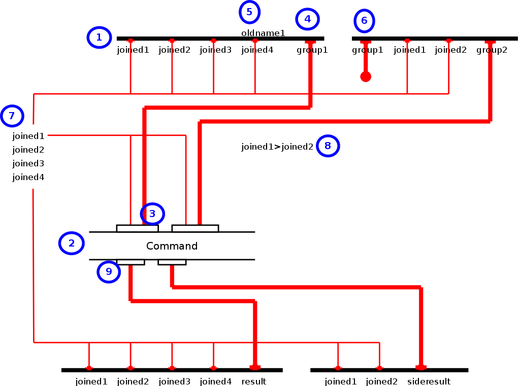
Figure 4. Example Flow Graph
Image 4 shows how a number of places and transitions are visualized. (1) Places are visualized as horizontal thick black lines, each with a list of attributes. (2) Commands are visualized as the name of the command between two thin black lines. The top side of the command contains the input ports (3) and the output ports (9). The input ports (3) take inputs from either grouped attributes from the places (4) or directly from one of the joined attributes (7). (5) Renames in the diagram are shown integrated into the places. If an attribute is listed both above and under the place line it annotates that the attribute oldname1 is renamed to joined4. (6) Grouped attributes which are not used are marked as dead end attributes through a thick red line which ends in a circle. (4) Normal grouped attributes are marked through a thick red line. (9) the output of a command is always a red thick line since we use the full aggregate tab separated file. (7) all the attributes that contribute to the primary key and thus to the joining of the inputs are listed to the left. From there on they can further be used as inputs into the command or directly into the output places. (8) The guard that describes which combinations are allowed is written next to the command where there is place.
The advantage of using this type of diagram is that one con directly read which command will be executed on which data groups (to be found in the list of joined attributes (7)). One can also directly see how the rejoining operation takes place.
5. Some practical considerations
5.1. A Join operation that preserves some grouped attributes
The standard semantics for a transition provides a full join operation, which has the advantage that we can join multiple tables easily without needing to resort to a specific syntactical form or so. If we for instance place 3 tables as input into an empty command then this command will generate the joined tables automatically. A problem is of course that we with such a join operation would loose the grouped attributed. Sometimes this might be unwanted. Therefore the implementation of a join operator that simply passes through each input to its output will effectively perform the join and retain the grouped attributes for that particular input.
The implementation of this particular join operation is quite simple. It simply copies each of the inputs to the outputs. Practically we can define a command Join which will simply state outputs=inputs.
The results is that we can write something as
Join(Input(images,images.groups), Output(marked_images,images.groups), Input(gels), Input(params,params.groups), Output(marked_params,params.groups));
Here, the input will be joined on all common attributes. However the first output will be a joined entity together with all the grouped attributes that were at the images place. The second output will be the joined input merged into the grouped attributes of the params place.
5.2. Source places
Certain places are used to place information into a FlowPipe setup. E.g: providing images or entering data. This means that these places can be modifie in a non-functional manner, which in turn means that some form of change-detection of input modification must be present. This can be for instance the timestamps of files or the creation of new filenames and modification of meta-data. The later is very likely a better candidate than the former.
5.3. Caching
The execution of a transition happens such that it appears as if the output places are emptied before the transition starts executing all commands. After execution of the commands the output place contains all the output tokens. If we have multiple transitions which use the same output place then the behavior is similar as if each of the transitions would have their own output place and that we make the union of all these outputs.
Because it is imperformant to recalculate everything everytime a change to an input takes place, it is in general better to have some form of caching present that will not recalculate a certain command if the inputs did not change and the calculation was already performed in the past.
5.4. Intermediate places and persistent storage
The user should be able to observe the content of each place. As such, the data should remain persistent in a database or somewhere on the filesystem. This also means that all intermediate objects generated in the pipeline must remain available. Since this is often unwanted it is possible to mark places as intermediate. In that case the various files are removed when calculations are finished and meta data can also be removed. Whenever necessary the inputs can be indirectly retrieved again.
5.5. Parallelism
A transition is responsible for converting all its inputs into outputs. The order in which this is done is undefined. A transition can perform this process by spawning multiple concurrent processes, each dealing with the conversion of one token to the next. Of course, when a token refers to a file or so then this file must be accessible to the spawned command, meaning that if client machines are involved each of those machines must have access to the same filesystem.
5.6. Scheduling
5.6.1. Transition execution
In general a downstream transition should not be executed before all its upstream transitions have finished. The argument for this is that it might lead to unnecessary calculations. E.g: a transition generates images and dumps them in an output place which then regroups this data. The data group is then put into the next transition. However, every time the upstream transition finished a command it will extend this group and the downstream transition needs to be restarted. This might not be harmful and might even be wanted. Then one can observer the intermediate results downstream rather directly. However, sometimes it might be too time or disk space consuming to consider this. As such, scheduling must be decided by the user. Does (s)he wants to wait for the upstream calculations to finish or not ?
5.6.2. Potential tokens
Of course, when the system is capable of predicting in advance that there will be no more tokens of a specific type (because for instance the command output does not touch any potential of the input requirements of the downstream calculation), then it is possible to start interweaving the calculations. It is also possible to already reserve output tokens without content and declare that they might be calculated. This offers a great possibility where the user can already browse the potential output and select the tokens heshe is interested in.
5.6.3. Demand driven calculation
The system we presented has the advantage that it has no loops and thus to a certain extent it can deal with calculations in a demand driven fashion. If a transition requires all combinations of a specific token to be present then the inputs can be required to generate exactly tokens of this type. This of course goes only so far. If the type of token that is required is the result of the direct output of a command it is fairly impossible to predict how it can be obtained. In that case all combinations must be finished first. However, when this is not the case one can declare a required token at an output and transfer that knowledge to the input and prioritize the execution of each of the transitions.
6. A FlowPipes Implementation
Implementation wise we need the possibility to describe the different input states as well as the different commands. A command takes an input and an output. As a demonstration of the good working of this model we use C++ in which a command is a class which accepts multiple input tables and produces a number of output tables. If this is done on disk or directly in a database matters little to show the power of this model.
The implementation below is far from optimal but manages to capture all semantics properly. There are many places where distinctive improvements are possible. Especially in the joining of places as well as in the passing of tokens and the different views. Instead of copying all elements a form a pass by reference and copy on write would have been possible. That would however have made the implementation much less readable.
Tokens
struct Token
{
  int sx, sy;  // number of columns and rows
  void set_xy(int x, int y, string g);  // set column x and row y to value g
  string xy(int x, int y); // retrieve the content of column x and row y
};
Commands
class Command
{
  vector<Token> inputs,outputs;  // the input and output vectors
  /**
   * Set the input/output number argnr to token t
   */
  void set_input(unsigned int argnr, Token t);
  void set_output(unsigned int argnr, Token t);
  /**
   * The exexcute routine must execute the command on the provided inputs
   * and place the result in the outputs through set_output.
   */
  virtual void execute()=0;
};
Places
struct Place
{
  // the content as  an attribute to column mappign
  map<string, vector<string> > *content;
  // which attributes are marked as a group ?
  set<string> groups;
  // The rename operation will generate a new place where attribute
  // a is renamed to b
  Place rename(string a, string b);
  // get rid of a specific attribtue
  Place forget(string a);
  // add an element to this place. A record is a map of attributes to values
  void operator +=(map<string,string> r);
  // initialize a place with a number of atttributes
  Place(string a, string b, string c);
  // return the content of a particulat attribute
  vector<string>& operator[](string attr);
  // return the list of all attributes
  set<string> attrs();
};
Join
void execute(Command* cmd, vector<PlaceSelection> inputs, vector<PlaceSelection> outputs)
{
  // ----------------------------------------------
  // Step 1: obtaining the primary passthrough key
  // ----------------------------------------------
  set<string> primary_header;
  for(int i = 0 ; i < inputs.size(); i++)
    {
      set<string> S=inputs[i].place.attrs();
      for(set<string>::iterator it=S.begin(); it!=S.end(); it++)
	primary_header.insert(*it);
    }
  for(int i = 0 ; i < inputs.size(); i++)
    {
      set<string> S=inputs[i].place.groups;
      for(set<string>::iterator it=S.begin(); it!=S.end(); it++)
	primary_header.erase(*it);
    }

   //-------------------------------------------------
   // Step 2: Find potential useable combinations
   //-------------------------------------------------
  vector<int> combination_number;
  set< map<string,string> > proper_combinations;
  for(int i = 0 ; i < inputs.size(); i++)
    {
      combination_number.push_back(0);
      assert(inputs.size()>0); // otherwise joins make no sense
    }
  bool increased=true;
  while(increased)
    {
      /**
       * for each of the attributes in the header we should verify that there
       * is no offending value present
       */
      bool reject_combination=false;
      map<string,string> combination_description;
      for(set<string>::iterator i = primary_header.begin() ;
	  i != primary_header.end() && !reject_combination; i++)
	{
	  string attr=*i;
	  /**
	   * Check for attr whether all the input places actually
	   * have this attribute and have the same value
	   */
	  bool valset=false;
	  string target_val;
	  for(int j = 0 ; j < inputs.size() && !reject_combination; j++)
	    {
	      if (inputs[j].place.has(attr))
		{
		  string val=inputs[j].place[attr][combination_number[j]];
		  if (valset)
		    {
		      if (val!=target_val)
			{
			  reject_combination=true;
			  break;
			}
		    }
		  else
		    {
		      target_val=val;
		      valset=true;
		    }
		  combination_description[attr]=val;
		}
	    }
	}
      if (!reject_combination)
	{
	  proper_combinations.insert(combination_description);
	}
      increased=false;
      int current_digit=0;
      while(!increased)
	{
	  if(current_digit>=inputs.size())
	    break;
	  if (++combination_number[current_digit]==
	      inputs[current_digit].place.size())
	    combination_number[current_digit]=0;
	  else
	    increased=true;
	  ++current_digit;
	}
    }

  //-------------------------------------------------
  // Step 3: Check the guard
  //-------------------------------------------------
  // ...


  //-------------------------------------------------
  // Step 4: execute the commands
  //-------------------------------------------------
  for(set<map<string,string> >::iterator it=proper_combinations.begin();
      it!=proper_combinations.end(); it++)
    {
      // Step 4a: obtain the token for the combination
      map<string,string> record=*it;
      vector<vector<int> > tokens;
      for(int i = 0 ; i < inputs.size(); i++)
	{
	  vector<int> rows;
	  for(int j = 0; j < inputs[i].place.size(); j++)
	    {
	      bool rowmatches=true;
	      for(map<string,string>::iterator jt=record.begin();
		  jt!=record.end() && rowmatches; jt++)
		if (inputs[i].place.has(jt->first))
		  {
		    if (inputs[i].place[jt->first][j]!=jt->second)
		      rowmatches=false;
		  }
	      if (rowmatches)
		rows.push_back(j);
	    }
	  tokens.push_back(rows);
	}

      // Step 4b: create the tokens for the command
      for(int i = 0 ; i < inputs.size(); i++)
	{
	  vector<int> rows = tokens[i];
	  vector<string> selected=inputs[i].selection;
	  Token token;
	  for(int j = 0 ; j < selected.size(); j++)
	    for(int k = 0 ; k < rows.size(); k++)
	      {
		string value = inputs[i].place[selected[j]][rows[k]];
		token.set_xy(j,k,value);
	      }
	  cmd->set_input(i,token);
	}

      // Step 4c: execute the command
      cmd->execute();

      // Step 4d: rejoin the output of the command
      for(int i = 0 ; i < outputs.size(); i++)
	{
	  vector<string> retrieved=outputs[i].selection;
	  Token token=cmd->outputs[i];
	  for(map<string,string>::iterator it=record.begin();
	      it!=record.end(); it++)
	    outputs[i].place[it->first];
	  for(int j = 0 ; j < retrieved.size(); j++)
	    outputs[i].place[retrieved[j]];

	  for(map<string,string>::iterator it=record.begin();
	      it!=record.end(); it++)
	    for(int k = 0 ; k < token.sy; k++)
	      outputs[i].place[it->first].push_back(it->second);
	  for(int j = 0 ; j < retrieved.size(); j++)
	    {
	      for(int k = 0 ; k < token.sy; k++)
		{
		  string value=token.xy(j,k);
		  if (record.find(retrieved[j])!=record.end())
		    assert(value==record[retrieved[j]]);
		  else
		    outputs[i].place[retrieved[j]].push_back(value);
		}
	    }
	}
    }
}
The above join operation is rather extensive. Since it is a very important operation which grasps the entire semantics, including reintegration of data, joining of the inputs we investigate each of the distinct steps involved. Step 1 determines which attributes should be the same across inputs. Because we will be working with attributes that are passed through and attributes that we won't we first need to obtain a list of attributes that are joinable.
1. An attribute is only passed through if it is not grouped in any of the inputs.
2. An attribute that appears non grouped in only one input will also be passed through as a primary key.
In step 2 we generate all combinations of input tokens. This routine is highly inefficient. It does however do a good job in explaining the semantics of the join operation. The routine will generate each potential combination and verify whether all the inputs have the same value. If there is no reason to reject a particular combination it is remembered in the proper_combinations set. In Step 3 we could go through each of the combinations using a declared guard. This is something we don't do however at the moment. In step 4 we will for each proper input combination execute the command and rejoin the commands' output into the target place together with the required fields from the primary key. If the output of the command didn't produce anything (and empty token) then no rejoining takes place since there is nothing to join against. As a potential improvement whenever no input is selected for a command, then the command must not be started since it has no bearing to the calculations in question. This fourth step will first obtain the full tokens for that particular combination (Step 4a). From these tokens a stripped down version is produced which are used as input into the command execution (Step 4b). Once these are created we execute the command (Step 4c). In the last substep (step 4d) we rejoin the output of the command by merging in the old fields for each produced row of the output tokens. If a field from the output should be placed in a column which was supposed to be passed through then the values must be the same.
7. The P53 Example
We want to have an example with the different images and patient parameters. The layout is relatively simple. Each patient has multiple gels. Each of these gels was acquired by a specific technician using a specific technique and often replicas were made, resulting in two different images (E.g New 1 and New2 tags) Each patient has multiple tests each resulting in a different number. Each gel belongs to a certain gel collection, for each combination of gel collection and parameter we want to generate a correlation image across all patients.
7.1. Source places
7.1.1. Images(patient,image*)
The images place keeps track of each patient and the gel images we obtained for them. For example we could have
  patient  image
  WVB      nicegel1
  WVB      nicegel2
  WVB      gel-XR
  WVB      gel-old
  WVB      gel-old2
  KTY      badgel1
  KTY      badgel2
  KTY      badoldgel2
  KTY      Xrayedkty
7.1.2. Gels(image*,gelgroup)
This place keeps track of which image belongs to which type of gel. We can have gels that belong to the New set (New1 or New2) or to the X-ray set or to the Old set. Interesting here is that certain gels belong to multiple groups at the same time. For instance a gel that belongs to the New1 or New2 group also directly belongs to the New group itself.
  nicegel1   New1
  nicegel2   New2
  gel-XR     XR
  gel-old    Old1
  gel-old2   Old2
  badgel1    New1
  badoldgel2 Old2
  badgel2    New2
  Xrayedkty  XR
  nicegel1   New
  nicegel2   New
  badgel1    New
  badgel2    New
  gel-old    Old
  gel-old2   Old
  badoldgel2 Old
  nicegel1   All
  nicegel2   All
  gel-XR     All
  gel-old    All
  gel-old2   All
  badgel1    All
  badoldgel2 All
  badgel2    All
  Xrayedkty  All
As illustration. Since the images attribute is a group attribute, we only have the following tokens
  nicegel1   New1
  badgel1    New1

  nicegel2   New2
  badgel2    New2

  gel-XR     XR
  Xrayedkty  XR

  gel-old    Old1

  gel-old2   Old2
  badoldgel2 Old2

  nicegel1   New
  nicegel2   New
  badgel1    New
  badgel2    New

  gel-old    Old
  gel-old2   Old
  badoldgel2 Old

  nicegel1   All
  nicegel2   All
  gel-XR     All
  gel-old    All
  gel-old2   All
  badgel1    All
  badoldgel2 All
  badgel2    All
  Xrayedkty  All
7.1.3. Params(patient,parameter,value)
This place keeps track of all the biological parameters we obtained for a patient. It maps the name of a patient together with a parameter to a value.
 WVB  survival         long
 WVB  health           great
 WVB  lifeexpectancy   128y
 KTY  health           fantastic
 KTY  lifeexpectancy   64y
Obviously these are nonsense values, half of them which are non numerical and thus cannot be correlated. That however does not matter in this example since we are mainly interested in demonstrating the type of combinations and data flow setup that can be created.
7.1.4. Preparing for correlation
The command we use to generate a correlation map will be called the Correlator. It takes one input: a tab separated file in which each row contains two elements. The first column is the name of the file that contains the image. The second column is a value that is associated with that particular image. In order now to correlate the proper datasets, we only need to generate for each patient and each biological parameter a combination. This means that we need to first join all images onto value. We can directly do this using the before mentioned Join command. The target place where we will dump this collection of data is MarkedImages(image*,value*,patient*, gelgroup, parameter). Normally the gelgroup and parameter arguments are automatically passed through and will extend the output place automatically.
 Join(Input(Images,Images.groups), Output(MarkedImages,Images.groups),
      Input(Gels),
      Input(Params,Params.groups));
If we run this operation on our dataset we get the following tokens in MarkedImages
gelgroup image* parameter patient* value*
All badgel1 health KTY fantastic
All badgel2 health KTY fantastic
All badoldgel2 health KTY fantastic
All Xrayedkty health KTY fantastic
All nicegel1 health WVB great
All nicegel2 health WVB great
All gel-XR health WVB great
All gel-old health WVB great
All gel-old2 health WVB great
All badgel1 lifeexpectancy KTY 64y
All badgel2 lifeexpectancy KTY 64y
All badoldgel2 lifeexpectancy KTY 64y
All Xrayedkty lifeexpectancy KTY 64y
All nicegel1 lifeexpectancy WVB 128y
All nicegel2 lifeexpectancy WVB 128y
All gel-XR lifeexpectancy WVB 128y
All gel-old lifeexpectancy WVB 128y
All gel-old2 lifeexpectancy WVB 128y
All nicegel1 survival WVB long
All nicegel2 survival WVB long
All gel-XR survival WVB long
All gel-old survival WVB long
All gel-old2 survival WVB long
New badgel1 health KTY fantastic
New badgel2 health KTY fantastic
New badoldgel2 health KTY fantastic
New Xrayedkty health KTY fantastic
New nicegel1 health WVB great
New nicegel2 health WVB great
New gel-XR health WVB great
New gel-old health WVB great
New gel-old2 health WVB great
New badgel1 lifeexpectancy KTY 64y
New badgel2 lifeexpectancy KTY 64y
New badoldgel2 lifeexpectancy KTY 64y
New Xrayedkty lifeexpectancy KTY 64y
New nicegel1 lifeexpectancy WVB 128y
New nicegel2 lifeexpectancy WVB 128y
New gel-XR lifeexpectancy WVB 128y
New gel-old lifeexpectancy WVB 128y
New gel-old2 lifeexpectancy WVB 128y
New nicegel1 survival WVB long
New nicegel2 survival WVB long
New gel-XR survival WVB long
New gel-old survival WVB long
New gel-old2 survival WVB long
New1 badgel1 health KTY fantastic
New1 badgel2 health KTY fantastic
New1 badoldgel2 health KTY fantastic
New1 Xrayedkty health KTY fantastic
New1 nicegel1 health WVB great
New1 nicegel2 health WVB great
New1 gel-XR health WVB great
New1 gel-old health WVB great
New1 gel-old2 health WVB great
New1 badgel1 lifeexpectancy KTY 64y
New1 badgel2 lifeexpectancy KTY 64y
New1 badoldgel2 lifeexpectancy KTY 64y
New1 Xrayedkty lifeexpectancy KTY 64y
New1 nicegel1 lifeexpectancy WVB 128y
New1 nicegel2 lifeexpectancy WVB 128y
New1 gel-XR lifeexpectancy WVB 128y
New1 gel-old lifeexpectancy WVB 128y
New1 gel-old2 lifeexpectancy WVB 128y
New1 nicegel1 survival WVB long
New1 nicegel2 survival WVB long
New1 gel-XR survival WVB long
New1 gel-old survival WVB long
New1 gel-old2 survival WVB long
New2 badgel1 health KTY fantastic
New2 badgel2 health KTY fantastic
New2 badoldgel2 health KTY fantastic
New2 Xrayedkty health KTY fantastic
New2 nicegel1 health WVB great
New2 nicegel2 health WVB great
New2 gel-XR health WVB great
New2 gel-old health WVB great
New2 gel-old2 health WVB great
New2 badgel1 lifeexpectancy KTY 64y
New2 badgel2 lifeexpectancy KTY 64y
New2 badoldgel2 lifeexpectancy KTY 64y
New2 Xrayedkty lifeexpectancy KTY 64y
New2 nicegel1 lifeexpectancy WVB 128y
New2 nicegel2 lifeexpectancy WVB 128y
New2 gel-XR lifeexpectancy WVB 128y
New2 gel-old lifeexpectancy WVB 128y
New2 gel-old2 lifeexpectancy WVB 128y
New2 nicegel1 survival WVB long
New2 nicegel2 survival WVB long
New2 gel-XR survival WVB long
New2 gel-old survival WVB long
New2 gel-old2 survival WVB long
Old badgel1 health KTY fantastic
Old badgel2 health KTY fantastic
Old badoldgel2 health KTY fantastic
Old Xrayedkty health KTY fantastic
Old nicegel1 health WVB great
Old nicegel2 health WVB great
Old gel-XR health WVB great
Old gel-old health WVB great
Old gel-old2 health WVB great
Old badgel1 lifeexpectancy KTY 64y
Old badgel2 lifeexpectancy KTY 64y
Old badoldgel2 lifeexpectancy KTY 64y
Old Xrayedkty lifeexpectancy KTY 64y
Old nicegel1 lifeexpectancy WVB 128y
Old nicegel2 lifeexpectancy WVB 128y
Old gel-XR lifeexpectancy WVB 128y
Old gel-old lifeexpectancy WVB 128y
Old gel-old2 lifeexpectancy WVB 128y
Old nicegel1 survival WVB long
Old nicegel2 survival WVB long
Old gel-XR survival WVB long
Old gel-old survival WVB long
Old gel-old2 survival WVB long
Old1 badgel1 health KTY fantastic
Old1 badgel2 health KTY fantastic
Old1 badoldgel2 health KTY fantastic
Old1 Xrayedkty health KTY fantastic
Old1 nicegel1 health WVB great
Old1 nicegel2 health WVB great
Old1 gel-XR health WVB great
Old1 gel-old health WVB great
Old1 gel-old2 health WVB great
Old1 badgel1 lifeexpectancy KTY 64y
Old1 badgel2 lifeexpectancy KTY 64y
Old1 badoldgel2 lifeexpectancy KTY 64y
Old1 Xrayedkty lifeexpectancy KTY 64y
Old1 nicegel1 lifeexpectancy WVB 128y
Old1 nicegel2 lifeexpectancy WVB 128y
Old1 gel-XR lifeexpectancy WVB 128y
Old1 gel-old lifeexpectancy WVB 128y
Old1 gel-old2 lifeexpectancy WVB 128y
Old1 nicegel1 survival WVB long
Old1 nicegel2 survival WVB long
Old1 gel-XR survival WVB long
Old1 gel-old survival WVB long
Old1 gel-old2 survival WVB long
Old2 badgel1 health KTY fantastic
Old2 badgel2 health KTY fantastic
Old2 badoldgel2 health KTY fantastic
Old2 Xrayedkty health KTY fantastic
Old2 nicegel1 health WVB great
Old2 nicegel2 health WVB great
Old2 gel-XR health WVB great
Old2 gel-old health WVB great
Old2 gel-old2 health WVB great
Old2 badgel1 lifeexpectancy KTY 64y
Old2 badgel2 lifeexpectancy KTY 64y
Old2 badoldgel2 lifeexpectancy KTY 64y
Old2 Xrayedkty lifeexpectancy KTY 64y
Old2 nicegel1 lifeexpectancy WVB 128y
Old2 nicegel2 lifeexpectancy WVB 128y
Old2 gel-XR lifeexpectancy WVB 128y
Old2 gel-old lifeexpectancy WVB 128y
Old2 gel-old2 lifeexpectancy WVB 128y
Old2 nicegel1 survival WVB long
Old2 nicegel2 survival WVB long
Old2 gel-XR survival WVB long
Old2 gel-old survival WVB long
Old2 gel-old2 survival WVB long
XR badgel1 health KTY fantastic
XR badgel2 health KTY fantastic
XR badoldgel2 health KTY fantastic
XR Xrayedkty health KTY fantastic
XR nicegel1 health WVB great
XR nicegel2 health WVB great
XR gel-XR health WVB great
XR gel-old health WVB great
XR gel-old2 health WVB great
XR badgel1 lifeexpectancy KTY 64y
XR badgel2 lifeexpectancy KTY 64y
XR badoldgel2 lifeexpectancy KTY 64y
XR Xrayedkty lifeexpectancy KTY 64y
XR nicegel1 lifeexpectancy WVB 128y
XR nicegel2 lifeexpectancy WVB 128y
XR gel-XR lifeexpectancy WVB 128y
XR gel-old lifeexpectancy WVB 128y
XR gel-old2 lifeexpectancy WVB 128y
XR nicegel1 survival WVB long
XR nicegel2 survival WVB long
XR gel-XR survival WVB long
XR gel-old survival WVB long
XR gel-old2 survival WVB long
This place has grouped attributes for image, patient and value, which leaves the gelgroup and parameter as primary key. Hereby we have automatically created the proper data collection. For each combination of gelgroup (Old, New, All, New1, New2 etc.) and parameter we can start a correlator.
7.1.5. Correlating
To correlate the MarkedImages now we simply put MarkedImages into the Correlator
  Correlator(Input(MarkedImages,"image","value"),
             Output(result,"correlationmap","significance","mask","count"));
If we now trace which Correlator commands are executed we obtain the following list.
 =Execution of Correlator==================================
 badgel1         fantastic
 badgel2         fantastic
 badoldgel2      fantastic
 Xrayedkty       fantastic
 nicegel1        great
 nicegel2        great
 gel-XR          great
 gel-old         great
 gel-old2        great
 =Execution of Correlator==================================
 badgel1         64y
 badgel2         64y
 badoldgel2      64y
 Xrayedkty       64y
 nicegel1        128y
 nicegel2        128y
 gel-XR          128y
 gel-old         128y
 gel-old2        128y
 =Execution of Correlator==================================
 nicegel1        long
 nicegel2        long
 gel-XR          long
 gel-old         long
 gel-old2        long
 =Execution of Correlator==================================
 badgel1         fantastic
 badgel2         fantastic
 badoldgel2      fantastic
 Xrayedkty       fantastic
 nicegel1        great
 nicegel2        great
 gel-XR          great
 gel-old         great
 gel-old2        great
 =Execution of Correlator==================================
 badgel1         64y
 badgel2         64y
 badoldgel2      64y
 Xrayedkty       64y
 nicegel1        128y
 nicegel2        128y
 gel-XR          128y
 gel-old         128y
 gel-old2        128y
 =Execution of Correlator==================================
 nicegel1        long
 nicegel2        long
 gel-XR          long
 gel-old         long
 gel-old2        long
None of these commands know the primary key. However, once the command is finished its output is rejoined with the primary key that defined the token. The correlator at the moment just returns a random correlationmap name, significance name and maskname. This then leads to the following result place:
correlationmap count gelgroup mask parameter significanceThrough two simple operations we created all proper combinations and used a modular correlator command to generate the necessary images and so on.
r17767 9 All m17767 health s17767
r9158 9 All m9158 lifeexpectancy s9158
r39017 5 All m39017 survival s39017
r18547 9 New m18547 health s18547
r56401 9 New m56401 lifeexpectancy s56401
r23807 5 New m23807 survival s23807
r37962 9 New1 m37962 health s37962
r22764 9 New1 m22764 lifeexpectancy s22764
r7977 5 New1 m7977 survival s7977
r31949 9 New2 m31949 health s31949
r22714 9 New2 m22714 lifeexpectancy s22714
r55211 5 New2 m55211 survival s55211
r16882 9 Old m16882 health s16882
r7931 9 Old m7931 lifeexpectancy s7931
r43491 5 Old m43491 survival s43491
r57670 9 Old1 m57670 health s57670
r124 9 Old1 m124 lifeexpectancy s124
r25282 5 Old1 m25282 survival s25282
r2132 9 Old2 m2132 health s2132
r10232 9 Old2 m10232 lifeexpectancy s10232
r8987 5 Old2 m8987 survival s8987
r59880 9 XR m59880 health s59880
r52711 9 XR m52711 lifeexpectancy s52711
r17293 5 XR m17293 survival s17293
7.1.6. Extending the dataset
As a further example of the power of this approach. Let's add another distinguishing feature. Not only do we have patients, we also have patients which we followed up for many years. In this case we just need to add a year attribute to the Patient place. This will automatically be propagated into the MarkedImages table, where it will form part of the primary key. This will then go through the correlator command and also extend the Results place with this new parameter.
However, if we would have been interested in correlating regardless of this year attribute, the only thing we have to do is to mark the 'Year' attribute in the Patients place to be a grouped attribute. No other changes to the pipeline are necessary.
8. The qPCR Case
The quantitative PCR example is somewhat more complicated and pushes the limits of the model. IT is however worth noting that although it appears to be a simple problem, even writing this example in a standard programming language often entails surprisingly difficult mappings and intertwining of loops.
8.1. Source places
8.1.1. Wells(x,y,value*)
Keeps track of the measured value in well (x,y)
 value*          x               y
 12.2            0               0
 12.4            1               0
 12.9            2               0
 11.1            0               1
 11.5            1               1
 11.0            2               1
 14.5            0               2
 14.5            1               2
 13.4            2               2
 9.3             0               3
 8.6             1               3
 12.2            2               3
 39.2            0               4
 48.5            1               4
 52.3            2               4
 39.3            0               5
 28.6            1               5
 na              2               5
8.1.2. Genes(y,gene)
Keeps track of the probes listed at a specific position.
 gene            y
 BRCA            0
 HH1             1
 BRCA            2
 HH1             3
 FKRP            4
 FKRP            5
8.1.3. CellSystem(y,cells)
Lists the different cell systems involved
 cells           y
 wt              0
 wt              1
 tg              2
 tg              3
 tg              4
 wt              5
8.1.4. Household(gene,household)
Keeps track of whether a specific gene can be used as a household gene or not
 gene            household
 BRCA            false
 FKRP            false
 HH1             true
8.2. Joining the inputs
Now it becomes tricky. Because the operation is inherently
difficult: that is to say the calculation involves 4 sets of data.
First we need to calculate the difference from the gene of interest to
the household gene, and this needs to be done for the two cell systems.
This means that we need a full join of all the inputs we have and then
calculate the value between the proper elements.
The first operation will fully join all data we have and aggregate the values and x'es.
 Join(Input(wells,"value","x"), Output(fulljoin,"value","x"),
      Iput(genes),
      Input(cellsystem),
      Input(household));
which leads to the following fulljoin place:
 cells           gene            household       value*          x*              y
 tg              BRCA            false           14.5            0               2
 tg              BRCA            false           14.5            1               2
 tg              BRCA            false           13.4            2               2
 tg              FKRP            false           39.2            0               4
 tg              FKRP            false           48.5            1               4
 tg              FKRP            false           52.3            2               4
 tg              HH1             true            9.3             0               3
 tg              HH1             true            8.6             1               3
 tg              HH1             true            12.2            2               3
 wt              BRCA            false           12.2            0               0
 wt              BRCA            false           12.4            1               0
 wt              BRCA            false           12.9            2               0
 wt              FKRP            false           39.3            0               5
 wt              FKRP            false           28.6            1               5
 wt              FKRP            false           na              2               5
 wt              HH1             true            11.1            0               1
 wt              HH1             true            11.5            1               1
 wt              HH1             true            11.0            2               1
8.3. Which combinations do we want to calculate
The calculation of the difference of value between the gene of interest (in this case this could be anything which is not a household gene) and a household gene is the first task. The command we have to our disposal is the Dct command. We first however need to create two new places. The first which will contain only the household genes. The second one which will only contain the non household genes.
  Place hh=fulljoin.where("household","true").forget("household").forget("y");
  Place ge=fulljoin.where("household","false").forget("household").forget("y");
Once these are created we want to create the proper inputs into the Dct command; a command which takes two inputs (not one). It is namely possible that we have slightly more measurements for one gene than for the other. As such is it necessary to take the mean of the input values before we subtract them. In other words: it makes no sense to subtract first and then take the mean. Because putting place hh and ge directly into the Dct command would lead to a joining of all common attributes, in particular also on the genes. Because in the end we will want to compare one gene against the household gene, we also need to prepare this somewhat:
  Place ge1=ge.rename("gene","gene1").rename("cells","cells1");
  Place ge2=ge.rename("gene","gene2").rename("cells","cells2");
  Place hh1=hh.rename("gene","hh").rename("cells","cells1");
  Place hh2=hh.rename("gene","hh").rename("cells","cells2");
These are then directly joined and will effectively generate a list of
  Join(Input(ge1,"cells1"),
       Input(hh1),
       Input(ge2),
       Input(hh2),
       Output(required,"cells1"));
which gives all possible things we can calculate
 cells1          cells2          gene1           gene2           hh
 tg              tg              BRCA            BRCA            HH1
 tg              tg              BRCA            BRCA            HH1
 tg              tg              BRCA            BRCA            HH1
 tg              tg              BRCA            FKRP            HH1
 tg              tg              BRCA            FKRP            HH1
 tg              tg              BRCA            FKRP            HH1
 tg              tg              FKRP            BRCA            HH1
 tg              tg              FKRP            BRCA            HH1
 tg              tg              FKRP            BRCA            HH1
 tg              tg              FKRP            FKRP            HH1
 tg              tg              FKRP            FKRP            HH1
 tg              tg              FKRP            FKRP            HH1
 tg              wt              BRCA            BRCA            HH1
 tg              wt              BRCA            BRCA            HH1
 tg              wt              BRCA            BRCA            HH1
 tg              wt              BRCA            FKRP            HH1
 tg              wt              BRCA            FKRP            HH1
 tg              wt              BRCA            FKRP            HH1
 tg              wt              FKRP            BRCA            HH1
 tg              wt              FKRP            BRCA            HH1
 tg              wt              FKRP            BRCA            HH1
 tg              wt              FKRP            FKRP            HH1
 tg              wt              FKRP            FKRP            HH1
 tg              wt              FKRP            FKRP            HH1
 wt              tg              BRCA            BRCA            HH1
 wt              tg              BRCA            BRCA            HH1
 wt              tg              BRCA            BRCA            HH1
 wt              tg              BRCA            FKRP            HH1
 wt              tg              BRCA            FKRP            HH1
 wt              tg              BRCA            FKRP            HH1
 wt              tg              FKRP            BRCA            HH1
 wt              tg              FKRP            BRCA            HH1
 wt              tg              FKRP            BRCA            HH1
 wt              tg              FKRP            FKRP            HH1
 wt              tg              FKRP            FKRP            HH1
 wt              tg              FKRP            FKRP            HH1
 wt              wt              BRCA            BRCA            HH1
 wt              wt              BRCA            BRCA            HH1
 wt              wt              BRCA            BRCA            HH1
 wt              wt              BRCA            FKRP            HH1
 wt              wt              BRCA            FKRP            HH1
 wt              wt              BRCA            FKRP            HH1
 wt              wt              FKRP            BRCA            HH1
 wt              wt              FKRP            BRCA            HH1
 wt              wt              FKRP            BRCA            HH1
 wt              wt              FKRP            FKRP            HH1
 wt              wt              FKRP            FKRP            HH1
 wt              wt              FKRP            FKRP            HH1
It is possible to take tg(cells1)/BRCA(gene1) and compare it against
wt(cells2)/FKRP(gene2) based on household gene HH1. Of course from this
entire list we might want to weed out those that we don't want. For
instance we could demand that gene1 and gene2 are always the same. In
that case we can simply omit the renaming of gene to gene1/gene2. Or we
could use another input source that actually lists the combinations we
want to calculate. In any case, once we have this table we only nee dot
use it to generate the proper values that are put into the
calculator.
8.4. Calculating the
values
Given the list of required calculations in the Required place we can
now start calculating the
values.
  Dct(Input(ge1,"value"),
      Input(hh1,"value"),
      Input(required.forget("cells2").forget("gene2")),
      Output(system1,"gene1-dct"));
  Dct(Input(ge2,"value"),
      Input(hh2,"value"),
      Input(required.forget("cells1").forget("gene1")),
      Output(system2,"gene2-dct"));
In this case Dct will be called a number of times with the following value. The vertical line indicates that the two columns are independent inputs. This is also obvious since column 2 repeats in various combinations against column 1.
 14.5            |               9.3
 14.5            |               8.6
 13.4            |               12.2

 39.2            |               9.3
 48.5            |               8.6
 52.3            |               12.2

 12.2            |               11.1
 12.4            |               11.5
 12.9            |               11.0

 39.3            |               11.1
 28.6            |               11.5
 na              |               11.0
which leads to the System1 and System2 places.
 cells1          gene1           gene1-dct*      hh
 tg              BRCA            kaplah          HH1
 tg              FKRP            kaplah          HH1
 wt              BRCA            kaplah          HH1
 wt              FKRP            kaplah          HH1

 cells2          gene2           gene2-dct*      hh
 tg              BRCA            kaplah          HH1
 tg              FKRP            kaplah          HH1
 wt              BRCA            kaplah          HH1
 wt              FKRP            kaplah          HH1
8.5. Calculating the
values
 Dct(Input(system1,"gene1-dct"),
     Input(system2,"gene2-dct"),
     Input(required),
     Output(result,"ddct"));
which leads then to the following Result place:
 cells1          cells2          ddct            gene1           gene2           hh
 tg              tg              kaplah          BRCA            BRCA            HH1
 tg              tg              kaplah          BRCA            FKRP            HH1
 tg              tg              kaplah          FKRP            BRCA            HH1
 tg              tg              kaplah          FKRP            FKRP            HH1
 tg              wt              kaplah          BRCA            BRCA            HH1
 tg              wt              kaplah          BRCA            FKRP            HH1
 tg              wt              kaplah          FKRP            BRCA            HH1
 tg              wt              kaplah          FKRP            FKRP            HH1
 wt              tg              kaplah          BRCA            BRCA            HH1
 wt              tg              kaplah          BRCA            FKRP            HH1
 wt              tg              kaplah          FKRP            BRCA            HH1
 wt              tg              kaplah          FKRP            FKRP            HH1
 wt              wt              kaplah          BRCA            BRCA            HH1
 wt              wt              kaplah          BRCA            FKRP            HH1
 wt              wt              kaplah          FKRP            BRCA            HH1
 wt              wt              kaplah          FKRP            FKRP            HH1
Interestingly enough, if we would add another potential household gene, which was measured on the slide then we would automatically receive calculations based on such household gene as well.
9. Conclusions
Our FlowPipe system offers the following advantages:
1. Modular design. It is easy to add new pieces of information under the form of new attributes which are automatically propagated whether we want to use this attribute as a joinable attribute later on or not.
2. Natural development cycle: inspection of data and selection of grouped attributes make it fairly easy to modify the various potential combinations
3. The use of potential tokens make it possible to create results on demand.
4. The functional style brings both caching as well as persistency within the framework.
5. FlowPipes provides a directed acyclic graph through which data flows, making it easier to understand what leads to what in the final result.
6. New commands can be easily written and these commands do not need to know in what context the data is used.
7. Limited number of concepts. We have transitions, guards, commands, places and attributes. These are further extended with the important rename operator and group operator.
10. Acknowledgments
The idea behind this abstraction was created in 2005 to 2007, while working for Norut IT, in cooperation with Haukeland University Hospital and while working for LabForum, Medical Geneitcs, University of Tromsø. A half working implementation, which heavily relied on MySql, saw daylight at MedGen, but it was too slow and still had some missing semantics. In 2009 I finished the semantics and wrote it down.
Bibliography
| 1. | Correlation analysis of two-dimensional gel electrophoretic protein patterns and biological variables Werner Van Belle, Nina Ånensen, Ingvild Haaland, Oystein Bruserud, Kjell-Arild Høgda, Bjørn Tore Gjertsen BMC Bioinformatics; volume 7; nr 198; April 2006 http://werner.yellowcouch.org/Papers/2dcor/index.html |
| 2. | 2D Correlation Analysis Overview Werner Van Belle Yellowcouch Scientific; December 2007 http://analysis.yellowcouch.org/2dcor.html |
| 3. | Technical Report on Correlations: P53 Isoform Biosignatures vs Biomedical Parameters Werner Van Belle 93 Gb; February 2007 http://werner.yellowcouch.org/Papers/p53cor/ |
| 4. | Proteomics of p53 in Diagnostics and Therapy of Acute Myeloid Leukemia Nina Ånensen, Ingvild Haaland, Clive D'Santos, Werner Van Belle, Bjørn Tore Gjertsen Current Pharmaceutical Biotechnology; Bentham Science Publishers Ltd.; volume 7; nr 3; July 2006 http://werner.yellowcouch.org/Papers/p53proteo/index.html |
| 5. | Rule-based workflow management for bioinformatics John. S Conery, Julian M. Catchen, Michael, Lynch The VLDB Journal 14(3) 318-329; Springer Verlag; 14 October 2004; DOI 10.1007 s00778-005-0153-9 http://ix.cs.uoregon.edu/~conery/PDF/ConeryVLDB2005.pdf |
| 6. | Comunication by Means of Automata (Kommunikation mit Automaten). C.A. Petri |
| 7. | Petri Net Theory and the Modeling of Systems James L. Peterson Prentice-Hall, Englewood Cliffs, New Jersey, April 1981 |
| 8. | The Practitioner's Guide to Coloured Petri-nets Lars M. Kristensen, Soren Christensen, and Kurt Jensen International Journal on Software Tools for Technology Transfer (1998), 98-132 |
| http://werner.yellowcouch.org/ werner@yellowcouch.org |  |