| Home | Papers | Reports | Projects | Code Fragments | Dissertations | Presentations | Posters | Proposals | Lectures given | Course notes |
|
|
Correlation analysis of two-dimensional gel electrophoretic protein patterns and biological variablesWerner Van Belle1* - werner@yellowcouch.org, werner.van.belle@gmail.com Abstract : Background) Two-dimensional gel electrophoresis (2DE) is a powerful technique to examine post-translational modifications of complexly modulated proteins. Currently, spot detection is a necessary step to assess relations between spots and biological variables. This often proves time consuming and difficult when working with non-perfect gels. We developed an analysis technique to measure correlation between 2DE images and biological variables on a pixel by pixel basis. After image alignment and normalization, the biological parameters and pixel values are replaced by their specific rank. These rank adjusted images and parameters are then put into a standard linear Pearson correlation and further tested for significance and variance. Results) We validated this technique on a set of simulated 2DE images, which revealed also correct working under the presence of normalization factors. This was followed by an analysis of p53 2DE immunoblots from cancer cells, known to have unique signaling networks. Since p53 is altered through these signaling networks, we expected to find correlations between the cancer type (acute lymphoblastic leukemia and acute myeloid leukemia) and the p53 profiles. A second correlation analysis revealed a more complex relation between the differentiation stage in acute myeloid leukemia and p53 protein isoforms. Conclusion) The presented analysis method measures relations between 2DE images and external variables without requiring spot detection, thereby enabling the exploration of biosignatures of complex signaling networks in biological systems.
Keywords:
2D electrophoretic gels, correlation, 2D gel analysis, P53 FAB classifications, AML, ALL |
Table Of Contents
Background
Two-dimensional gel electrophoresis (2DE) has been a successful technique for identification and visualization of post-translational modifications [1](reviewed in [2]), and is increasingly used to determine accessible parts of the proteome in human cells [3]. To a certain extent has 2DE been used to propose diagnosis or clinical classification in diseases [4, 5, 6, 7, 8, 9], including differentiating acute myeloid leukemia (AML) from acute lymphoblastic leukemia (ALL) [10]. The amount and complexity of data obtained from 2DE patterns have led to the development of analysis software for digitalized images [11, 12, 13], but human interpretation and validation of the data is usually necessary. Typically, one of the steps in 2DE analysis is the selection of spots followed by description of their position, volume and other variables. Current methods for spot detection assume regular spot shapes [14]or model spots as bivariate Gaussian densities [15], and therefore cannot discriminate spot shapes and irregularity [16, 17]. In this paper we present a method that omits the spot detection phase and does not require human interpretation on a gel-to-gel basis.
Given a set of gel images, the technique measures correlation between every pixel position and an external variable. This makes it possible to study the 2DE protein distribution as well as the actual relation to the external variable. The method has been rigorously tested on a set of simulated 2DE images with different levels of background, additional noise and outliers. Biological evaluation of the technique was performed by testing the correlation analysis on p53 protein isoform profiles in cell samples from patients with well-characterized hematological malignancies.
Different hematological malignancies, like ALL and AML [18]are characterized by distinct mutations or expression of genes involved in cell signaling [19, 20]. The TP53 gene is frequently mutated in many cancers and mutations in signaling pathways acting on p53 protein are found both in sporadic and hereditary cancers [21]. The p53 protein is a sequence specific transcription factor that can regulate differentiation, growth and cell death, and is highly regulated by post-translational modifications caused by multiple signaling networks that directly or indirectly target the protein [22, 23]. During differentiation, p53 undergoes modifications like phosphorylation and acetylation and is suggested to be involved in differentiation of AML [24, 25]. Because of this large range of activities and complex regulatory functions, we relied on analysis of the post-translationally modified p53 protein to illustrate our method. The p53 protein biosignatures in 39 AML patients and 8 ALL patients were analyzed by 2DE immunoblot. Distinct p53 biosignatures correlated with cancer type (AML versus ALL) and, within the AML group, p53 biosignatures correlated with the level of differentiation, using the French-American-British (FAB) classification.
Results
Overview of the method
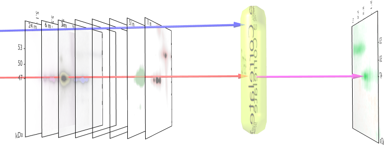 Figure 1 - 2DE Image Correlation 2DE image
correlation relies on an aligned, normalized stack of 2DE images and
a numerical label associated with every gel. Pixel per pixel
correlation between gel intensities (red arrow) and the external
variable (blue arrow) creates a new image, showing areas in the gel
that relate to the external parameter. In comparison to standard gel
analysis methods, spot detection is not necessary and therefore less
bias is introduced into the analysis process. This technique also
recognizes moving spots and spot shapes that
change. Click here for a movie of
the method
Figure 1 - 2DE Image Correlation 2DE image
correlation relies on an aligned, normalized stack of 2DE images and
a numerical label associated with every gel. Pixel per pixel
correlation between gel intensities (red arrow) and the external
variable (blue arrow) creates a new image, showing areas in the gel
that relate to the external parameter. In comparison to standard gel
analysis methods, spot detection is not necessary and therefore less
bias is introduced into the analysis process. This technique also
recognizes moving spots and spot shapes that
change. Click here for a movie of
the method
|
The presented method relies on the basic assumption that if spots
on 2DE images have biological relevance, then so must the pixels
comprised
within those spots. Therefore it must be possible to analyze 2DE images
for correlation, without performing a spot detection step. The method
requires the availability of a properly aligned stack of gel images.
Each of the images must have an associated parameter ![]() . Practically,
. Practically,
![]() can represent any biological
variable such as life expectancy,
differentiation stage of a cell sample, age of an organism, origin
of a cancer cell sample, effect of cancer therapy, cell size or even
variables such as time, temperature, pressure, and so on. For every
coordinate in the 2DE image stack, a correlation analysis is performed
between the pixel data gathered at that position and the external
variable
can represent any biological
variable such as life expectancy,
differentiation stage of a cell sample, age of an organism, origin
of a cancer cell sample, effect of cancer therapy, cell size or even
variables such as time, temperature, pressure, and so on. For every
coordinate in the 2DE image stack, a correlation analysis is performed
between the pixel data gathered at that position and the external
variable ![]() . The correlation image is
then created by repeating
this process at every possible position. The work-flow and the concept
behind the correlation method is illustrated in Fig. 1.
A movie of the method is available.
. The correlation image is
then created by repeating
this process at every possible position. The work-flow and the concept
behind the correlation method is illustrated in Fig. 1.
A movie of the method is available.
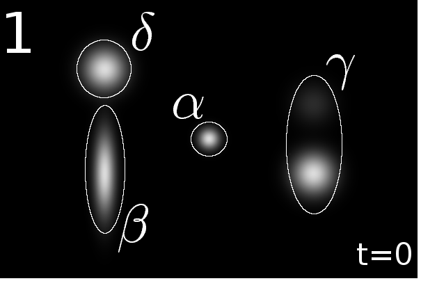
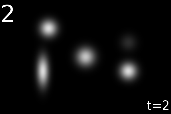
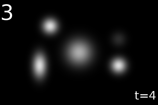
To illustrate how the correlation images ought to be interpreted,
a simulated gel stack with defined spot characteristics in function
of an external variable ![]() was
created (Fig. 2).
This simulation reassured a controlled environment in which the
algorithmic
behavior was observed.
was
created (Fig. 2).
This simulation reassured a controlled environment in which the
algorithmic
behavior was observed.
Simulated Gels
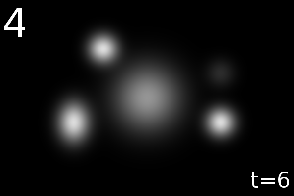
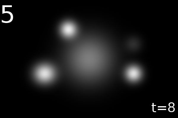
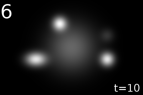
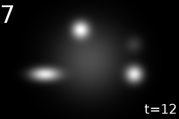
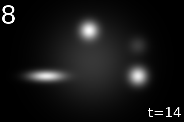
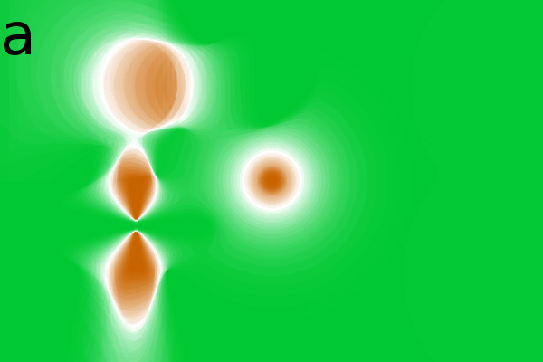
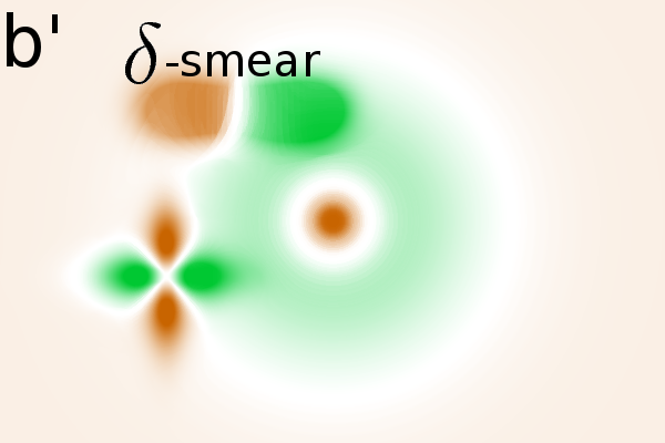
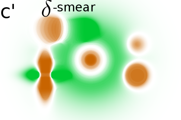
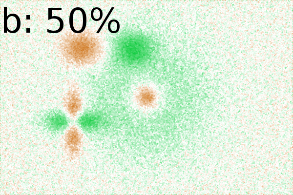
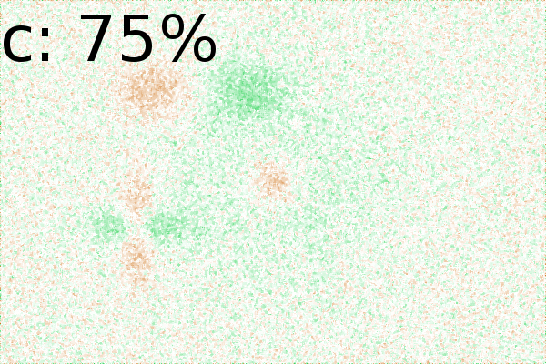
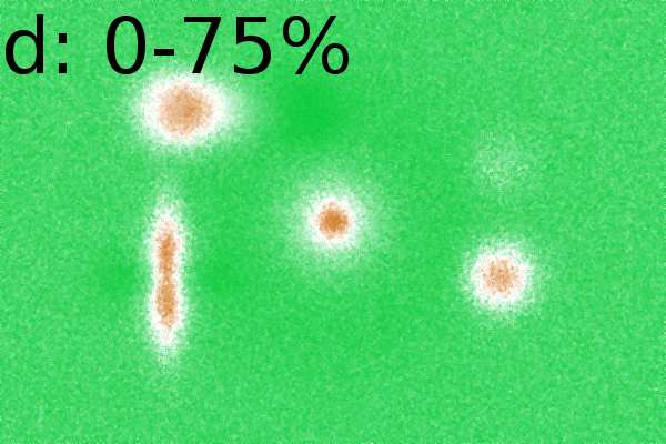
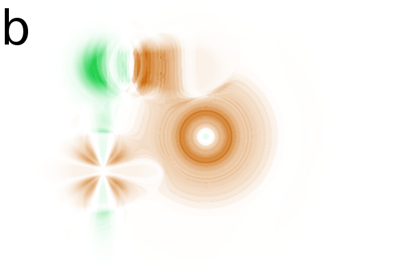
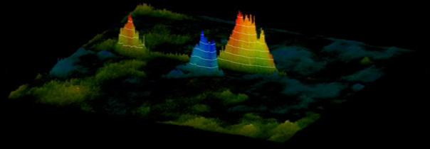
Figure 2 - Correlation towards a simulated 2DE gel-stack. (A) Eight snapshots taken from a stack of 15 simulated gels generated using Gaussian bumps. Each image contains simulated spots with particular characteristics. See Material and Methods for formula and details. (B) Correlation between the gel-stack and the variable | ||||||||||||||||||||||||||||||||||||||||||||||||||||||||||||||||||||||

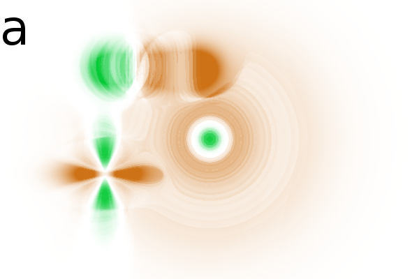

Altering spot position and sizes
We first verified how the method reacts to spot location, spot size
and spot shifts. The simulated gel stack has various spots behaving
differently. Spot ![]() grows and
fades out, spot
grows and
fades out, spot ![]() shifts
from left to right, spot
shifts
from left to right, spot ![]() changes shape and the
changes shape and the ![]() spots have a constant amplitude and width (Fig. 2A).
Fig
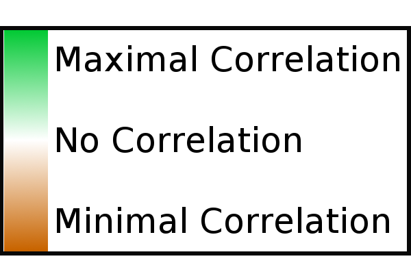
2 shows various correlation images in which
the
strength of a correlation is presented in shades of green (for positive
correlation) and brown (for negative correlation or anti-correlation).
By design, spots
spots have a constant amplitude and width (Fig. 2A).
Fig
2 shows various correlation images in which
the
strength of a correlation is presented in shades of green (for positive
correlation) and brown (for negative correlation or anti-correlation).
By design, spots ![]() and
and ![]() are parametrized by
are parametrized by ![]() .
In the correlation images (Fig. 2B) we find
them back
at the same position, showing that the correlation image offers correct
positional information. The two constant
.
In the correlation images (Fig. 2B) we find
them back
at the same position, showing that the correlation image offers correct
positional information. The two constant ![]() -spots are independent
of
-spots are independent
of ![]() . This results in no
visible correlation in Fig. 2Bab.
The
. This results in no
visible correlation in Fig. 2Bab.
The ![]() -spots shifts relates to
the external variable. The correlation
image reveals this by showing original and destination positions that
respectively correlate, then anti-correlate. This results in a smear
in the correlation image (Fig. 2B).
-spots shifts relates to
the external variable. The correlation
image reveals this by showing original and destination positions that
respectively correlate, then anti-correlate. This results in a smear
in the correlation image (Fig. 2B).
Spot shape
All images in Fig. 2B show the ![]() -spot to anti-correlate
in the middle and to correlate at its periphery. This is consistent
with the creation of the gel-stack in which the amplitude of spot
-spot to anti-correlate
in the middle and to correlate at its periphery. This is consistent
with the creation of the gel-stack in which the amplitude of spot
![]() lowers from 5.0 to 1.0
while the spots broadens from 10
to 100 pixels. Because the central spot widens, higher gel numbers
will have relatively more signal in the periphery. This indicates
that spots where diffusion-like alteration dominate can be detected
based on the difference in correlation between the inner and outer
areas. Similar behavior can be observed in the shape changing
lowers from 5.0 to 1.0
while the spots broadens from 10
to 100 pixels. Because the central spot widens, higher gel numbers
will have relatively more signal in the periphery. This indicates
that spots where diffusion-like alteration dominate can be detected
based on the difference in correlation between the inner and outer
areas. Similar behavior can be observed in the shape changing ![]() -spot.
The initial vertical shape (low
-spot.
The initial vertical shape (low ![]() -value)
anti-correlates
(it disappears)
while the later horizontal shape (at higher
-value)
anti-correlates
(it disappears)
while the later horizontal shape (at higher ![]() -values) correlates
(it appears).
-values) correlates
(it appears).
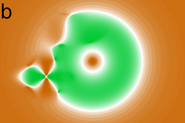
Masking the correlation image
In the simulated gel-stack, empty areas have an almost constant
intensity.
For those areas, the raw correlation analysis indicates a strong
correlation
(Fig. 2Ba) or anti-correlation (Fig. 2Bb).
There are two reasons for this. First, the area can be constant,
resulting
in correlations that are ![]() ,
,
![]() or NaN (not a number).
In the correlation image these are represented as +1 or -1. Secondly,
in areas with very small alterations (the periphery of the spots),
the measured correlation is mathematically correct, but the lack in
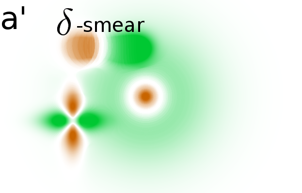
intensity variation offers little information. After applying various
significance masks to the correlation image, we find that only areas
with relevant spot modulations are indicated (Fig. 2B(a',b',c')).
One mask removes non significant correlations and a second mask removes
areas without variance (see Material and Methods, Step 4 for details).
or NaN (not a number).
In the correlation image these are represented as +1 or -1. Secondly,
in areas with very small alterations (the periphery of the spots),
the measured correlation is mathematically correct, but the lack in
intensity variation offers little information. After applying various
significance masks to the correlation image, we find that only areas
with relevant spot modulations are indicated (Fig. 2B(a',b',c')).
One mask removes non significant correlations and a second mask removes
areas without variance (see Material and Methods, Step 4 for details).
Effect of different normalizations
Different background removal and scaling techniques were tested on
the simulated gel-stack (Fig. 2), including
background
subtraction and background division. In all cases, the original
information
that led to the creation of the gel-stack was retrieved. The ![]() ,
,
![]() and
and ![]() spot correlations were always visualized,
indicating
that the normalization technique used is of little importance for
qualitative analysis. In the particular case of gel normalization
obtained by division through the mean gel intensity, new information
was found that did not directly originate from the creation of the
simulation (Fig. 2Bc). Due to a
spot correlations were always visualized,
indicating
that the normalization technique used is of little importance for
qualitative analysis. In the particular case of gel normalization
obtained by division through the mean gel intensity, new information
was found that did not directly originate from the creation of the
simulation (Fig. 2Bc). Due to a ![]() -dependent intensity
increase in spot
-dependent intensity
increase in spot ![]() , the mean
intensity of the gel increased.
As a result, the original constant
, the mean
intensity of the gel increased.
As a result, the original constant ![]() -spots decreased in intensity
(division by a larger number leads to lower values). The
-spots decreased in intensity
(division by a larger number leads to lower values). The ![]() -spots
became
-spots
became ![]() dependent and thus showed
up in the correlation image.
dependent and thus showed
up in the correlation image.
When working with real gels this does not hinder qualitative analysis because normalization is performed on an individual gel basis. Therefore, it can always be repeated on any new gel, without taking into account previous gels and the reported correlations can be observed in the normalized images. Quantitatively, normalization factors strongly influence correlation measures. If the technique is used as a quantitative method, then calibration spots ought to be used and exact understanding of machine specifications and camera properties should be known.
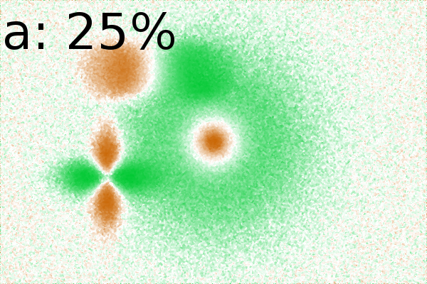
White noise in 2DE images
In Fig. 2Ba-c, the background correlated
towards ![]() .
Adding white noise [26]to
the simulated images
attenuates the appearance of such non significant background
correlations
(Fig. 2Ca-c). Increasing noise up to 75% (of
the
maximum image intensity) resulted in weaker correlations, but still
important spots were identifiable (Fig. 2Cc).
This
suggests
that small amounts of noise might enhance interpretation
of the correlation analysis by automatically introducing a
non-correlating
variance. The signal hidden within the noise must now compete against
a non-correlating factor, as such, the noise introduces a form of
automatic significance measurement. When the noise amplitude is
.
Adding white noise [26]to
the simulated images
attenuates the appearance of such non significant background
correlations
(Fig. 2Ca-c). Increasing noise up to 75% (of
the
maximum image intensity) resulted in weaker correlations, but still
important spots were identifiable (Fig. 2Cc).
This
suggests
that small amounts of noise might enhance interpretation
of the correlation analysis by automatically introducing a
non-correlating
variance. The signal hidden within the noise must now compete against
a non-correlating factor, as such, the noise introduces a form of
automatic significance measurement. When the noise amplitude is ![]() dependent, we observe correct information about the negative
correlation,
but loss of information about the positive correlation (Fig 2Cd).
Such a situation could occur if a camera automatically gates images
at waning signal strength. As long as white noise does not relate
to the external variable, its presence barely influences the analytical
power of the presented correlation test.
dependent, we observe correct information about the negative
correlation,
but loss of information about the positive correlation (Fig 2Cd).
Such a situation could occur if a camera automatically gates images
at waning signal strength. As long as white noise does not relate
to the external variable, its presence barely influences the analytical
power of the presented correlation test.
Effect of randomization of the dataset
Two sets of random data were generated to be used as ![]() -value. Instead
of testing correlation towards the sequence number
-value. Instead
of testing correlation towards the sequence number ![]() , we now determined
the effect of correlation of the images towards a random vector. The
IDL function 'randomu' [27],
generated
the normally
distributed random numbers. In the correlation images we always
recognized
the same general shapes. Areas that behaved similarly in the gel stack,
had the same coloring, regardless of the external variable. These
examples emphasize the robustness of the algorithm to group together
regions of interest (Fig. 2D).
, we now determined
the effect of correlation of the images towards a random vector. The
IDL function 'randomu' [27],
generated
the normally
distributed random numbers. In the correlation images we always
recognized
the same general shapes. Areas that behaved similarly in the gel stack,
had the same coloring, regardless of the external variable. These
examples emphasize the robustness of the algorithm to group together
regions of interest (Fig. 2D).
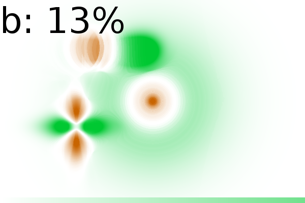
Outliers
A test with outliers in the ![]() -values
shows
limited impact on the
interpretation of the gels (Fig. 2E). We
changed the
-values
shows
limited impact on the
interpretation of the gels (Fig. 2E). We
changed the
![]() -values from {0, 1, 2, 3, 4, 5, 6, 7,
8, 9, 10, 11, 12, 13, 14}
to {0, 1, 15, 3, 4, 5, 6, 7, 8, 9, 10, 11,
12, 13, 14},
resulting in a slight change in actual correlation magnitude, but
the information content was well preserved. Even with 13% outliers
{0, 1, 15, 3, 4, 5, 6, 4, 8, 9, 10, 11, 12, 13,
14}, the original information was recovered. This is mainly due to
the robust correlation which relies on ranking of the dataset instead
of the numerical values (both the
-values from {0, 1, 2, 3, 4, 5, 6, 7,
8, 9, 10, 11, 12, 13, 14}
to {0, 1, 15, 3, 4, 5, 6, 7, 8, 9, 10, 11,
12, 13, 14},
resulting in a slight change in actual correlation magnitude, but
the information content was well preserved. Even with 13% outliers
{0, 1, 15, 3, 4, 5, 6, 4, 8, 9, 10, 11, 12, 13,
14}, the original information was recovered. This is mainly due to
the robust correlation which relies on ranking of the dataset instead
of the numerical values (both the ![]() -values and the image pixel
values are ranked).
-values and the image pixel
values are ranked).
Correlation analysis of p53 biosignatures in acute leukemia
Recently we demonstrated that signaling networks may be altered and potentiated in cancer cells suggesting a prognostic meaningful classification [28, 29]. This includes altered p38 MAP-kinase signaling, known to phosphorylate p53. The application of the presented method was tested on p53 biosignatures of human primary cancer cells. The p53 biosignature is probably formed by the combinations of splice forms of p53 and various post-translational modifications [22, 30]. The p53 protein is also involved in several positive and negative feedback networks [23]. This has ignited the hypothesis that p53 integrates information from various signaling networks [31].
We investigate two different relations. One illustrates a relation between the overall p53 intensity and AML/ALL classification, the other illustrates detection of p53-isoform biosignatures related to the AML FAB classification.
Correlation of p53 protein biosignatures towards AML/ALL
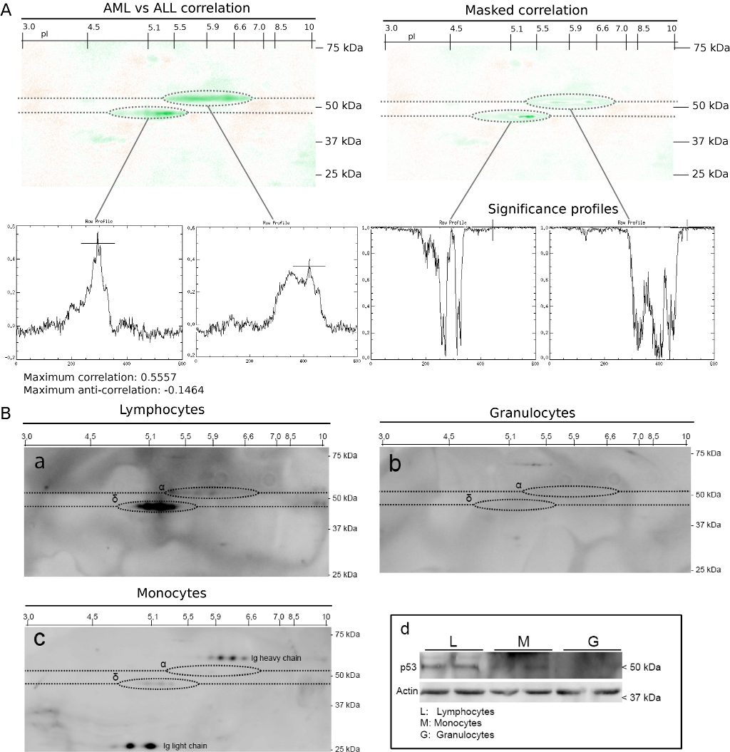 Figure 3 -
Correlation of p53 isoforms towards cancer type
(AML or ALL)
(A) Correlation analysis of p53 2DE immunoblots from AML and ALL
patient
samples. A total of 73 immunoblot images from AML and 16 images from
ALL were analyzed (left, correlation; right, masked correlation).
Green color indicates positive correlation for ALL (maximum positive
correlation 0.5557), and brown color indicates negative correlation
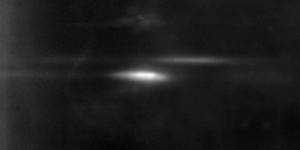
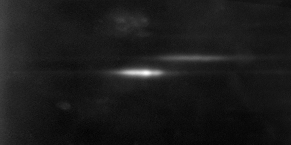
(maximum negative correlation 0.1464). (B) p53 protein expression
in mature lymphocytes, neutrophile granulocytes, and monocytes from
healthy donors, examined by 2DE (a-c) and one-dimensional immunoblot
(d). For comparison, protein extract from the different normal cell
types were analyzed by one-dimensional gel electrophoresis and
immunoblotting
(d). In the monocyte isolates, immunoglobulin subunits (heavy chain,
light chain) from the isolation procedure were detected in addition
to weak p53-
Figure 3 -
Correlation of p53 isoforms towards cancer type
(AML or ALL)
(A) Correlation analysis of p53 2DE immunoblots from AML and ALL
patient
samples. A total of 73 immunoblot images from AML and 16 images from
ALL were analyzed (left, correlation; right, masked correlation).
Green color indicates positive correlation for ALL (maximum positive
correlation 0.5557), and brown color indicates negative correlation
(maximum negative correlation 0.1464). (B) p53 protein expression
in mature lymphocytes, neutrophile granulocytes, and monocytes from
healthy donors, examined by 2DE (a-c) and one-dimensional immunoblot
(d). For comparison, protein extract from the different normal cell
types were analyzed by one-dimensional gel electrophoresis and
immunoblotting
(d). In the monocyte isolates, immunoglobulin subunits (heavy chain,
light chain) from the isolation procedure were detected in addition
to weak p53- |
ALL and AML comprise different genetic abnormalities
[32, 33], and analysis of growth
factor receptor expression and global gene expression has pointed out
that the expression of receptor tyrosine kinases and signaling
modulators are different [34, 35]. Therefore, since the p53 protein is implied in various cancer
related signaling networks, we expected to find distinct correlations
between p53 expression and the AML/ALL variable. Gels of AML patients
were marked with ![]() , while ALL
variants were marked with
, while ALL
variants were marked with ![]() .
The correlations are shown in Fig. 3A. It
reveals overall intensity attenuation of
p53 in AML compared to ALL. There is no previous data from acute
leukemia that supports this observation. To examine whether the 2DE
p53 correlations analysis reflected actual p53 protein expression
differences in the lymphoid and myeloid cell lineages, we examined
normal lymphocytes, neutrophile granulocytes and monocytes by 2DE
(Fig. 3Ba-c) and one-dimensional immunoblot
(Fig. 3d). This confirmed the
intensity-differences detected by the correlation analysis by
reflecting actual attenuated p53 protein levels in lymphocytes
compared to myeloid cells.
.
The correlations are shown in Fig. 3A. It
reveals overall intensity attenuation of
p53 in AML compared to ALL. There is no previous data from acute
leukemia that supports this observation. To examine whether the 2DE
p53 correlations analysis reflected actual p53 protein expression
differences in the lymphoid and myeloid cell lineages, we examined
normal lymphocytes, neutrophile granulocytes and monocytes by 2DE
(Fig. 3Ba-c) and one-dimensional immunoblot
(Fig. 3d). This confirmed the
intensity-differences detected by the correlation analysis by
reflecting actual attenuated p53 protein levels in lymphocytes
compared to myeloid cells.
|
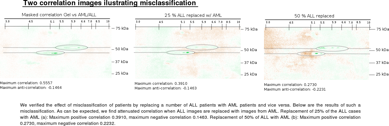
The impact of wrong ALL versus AML diagnosis was examined by random swapping ALL and AML labels in the AML/ALL versus 2DE image correlations. This results in lower correlation values as expected.
Correlation of p53 protein isoforms towards the AML differentiation level
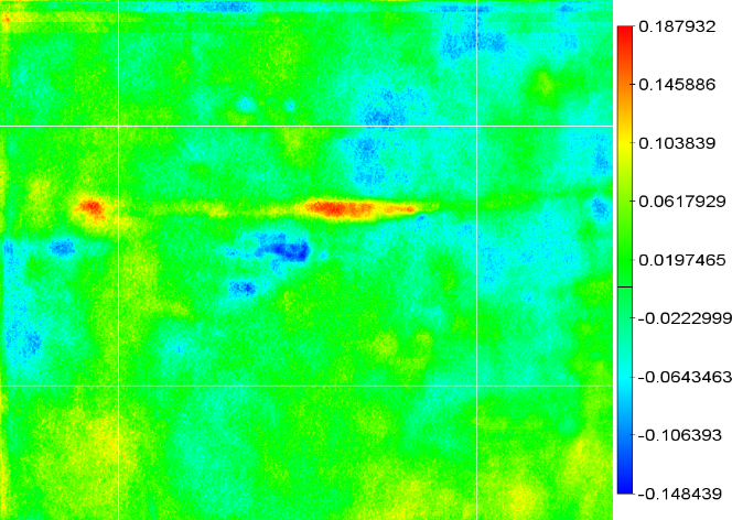
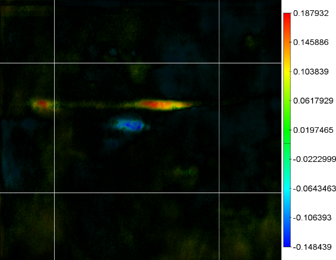
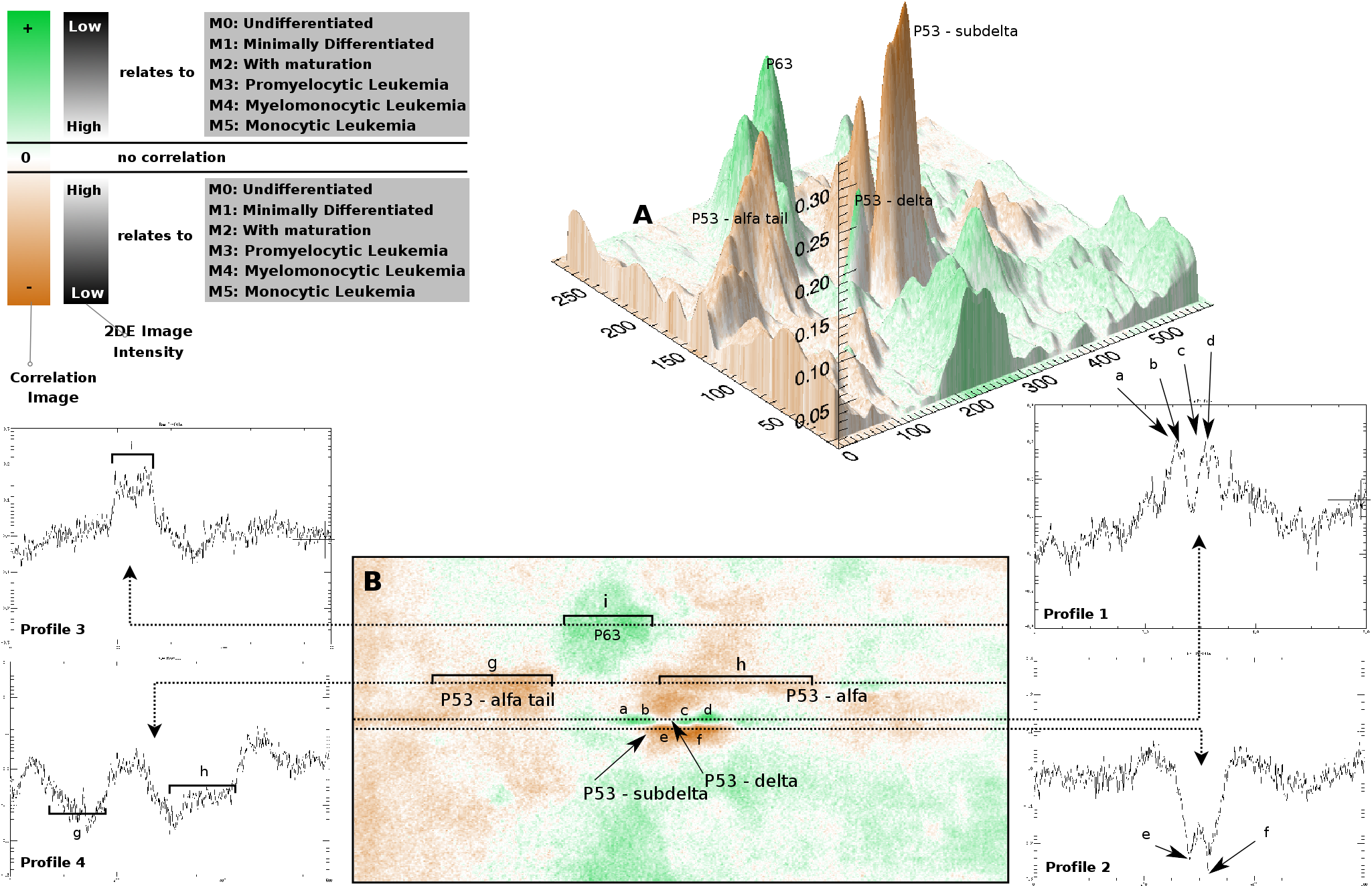 Figure 4 - Correlation of p53 protein isoforms towards
AML differentiation (FAB). Green indicates correlation
with more differentiated forms of AML. Such areas in 2DE
images of M5 will have a higher intensity than 2DE images of
M0. Brown indicates anti-correlation with the more mature forms
of leukemia cells. Such areas in 2DE images of M0 will have a
higher intensity than 2DE images of M5. (A) Correlation
landscape of p53 in 73 AML images related to differentiation
direction and stage (FAB, French-American-British
classification). The vertical axis sets out the absolute
correlation value. (B) Correlation image demonstrating
statistical significant alterations in p53. Profile 1 shows the
p53-
Figure 4 - Correlation of p53 protein isoforms towards
AML differentiation (FAB). Green indicates correlation
with more differentiated forms of AML. Such areas in 2DE
images of M5 will have a higher intensity than 2DE images of
M0. Brown indicates anti-correlation with the more mature forms
of leukemia cells. Such areas in 2DE images of M0 will have a
higher intensity than 2DE images of M5. (A) Correlation
landscape of p53 in 73 AML images related to differentiation
direction and stage (FAB, French-American-British
classification). The vertical axis sets out the absolute
correlation value. (B) Correlation image demonstrating
statistical significant alterations in p53. Profile 1 shows the
p53- |
The French-American-British (FAB) classification of AML is based on the morphologically determined stage of myeloid maturation and direction of maturation [36, 37]. Recent reports indicate that the FAB classification, in particular the distinction between M1-2 and M4-5 in maturation level and direction of maturation, is associated with certain gene classes in unsupervised clustering of gene expression profiles [38, 39]. It is previously described in several reports that p53 is involved in leukemic cell differentiation [24, 40, 25, 41]. Phosphorylation of p53 Ser315 is necessary for differentiation in mouse embryonic stem cells [42], and p53 is able to direct differentiation in AML cell lines [41, 25]. The p53-deficient HL-60 cell line has potential for both monocytic and granulocytic differentiation, and introduction of wild type p53 directs differentiation in the granulocytic direction [40]. Based on these reports we hypothesized that the p53 biosignatures should reflect the stage and direction of myeloid differentiation. Therefore, we measured correlations between the established routine morphological differentiation classification of AML (FAB) [21, 22, 35] and the p53 2DE biosignatures of the cancer cells.
We assigned to every class a separate ![]() -value: M0 (
-value: M0 (![]() ),
M1
(
),
M1
(![]() ), M2 (
), M2 (![]() ), M3 (
), M3 (![]() ),
M4 (
),
M4 (![]() ) and M5 (
) and M5 (![]() ). Using
73 gels we found specific correlations (Fig. 4).
Image
A
is the masked correlation landscape, image B is the raw correlation
image. The observations were: a) The tail of the p53-
). Using
73 gels we found specific correlations (Fig. 4).
Image
A
is the masked correlation landscape, image B is the raw correlation
image. The observations were: a) The tail of the p53-![]() isoform
correlates negatively to the FAB classification (profile 4, region
g and h). b) The p63 area correlates positively towards the FAB
classification
(profile 3, the i region). c) The p53-
isoform
correlates negatively to the FAB classification (profile 4, region
g and h). b) The p63 area correlates positively towards the FAB
classification
(profile 3, the i region). c) The p53-![]() region has four positively
correlating articulated spots (profile 1, a-d, r=0.2), d) the p53
sub-
region has four positively
correlating articulated spots (profile 1, a-d, r=0.2), d) the p53
sub-![]() region has two negatively
correlating spots (profile
2e,f). The combination of a positive correlation at the p53-
region has two negatively
correlating spots (profile
2e,f). The combination of a positive correlation at the p53-![]() region and a negative correlating sub-
region and a negative correlating sub-![]() region indicates a
spot shift from one area to another. Additionally, the e) presence
of the super-
region indicates a
spot shift from one area to another. Additionally, the e) presence
of the super-![]() negative
correlating region indicates that
a change of spot shape also occurs. When the p53-
negative
correlating region indicates that
a change of spot shape also occurs. When the p53-![]() spots are
larger and diffuse then the patient is classified as M0, M1 or M2.
If the spots in the
spots are
larger and diffuse then the patient is classified as M0, M1 or M2.
If the spots in the ![]() region are clear articulated and smaller,
the patient is either M4 or M5. None of the above correlations are
strong (
region are clear articulated and smaller,
the patient is either M4 or M5. None of the above correlations are
strong (![]() using the
stringent Spearman rank order correlation).
Nonetheless they can be observed in the 2DE images, which means that
they can form an important tool in stratification of patients. Based
on these correlation measurements, we performed further tests to verify
and confirm the relation between mass-differences and the FAB
classification (See section Intra-image correlations).
using the
stringent Spearman rank order correlation).
Nonetheless they can be observed in the 2DE images, which means that
they can form an important tool in stratification of patients. Based
on these correlation measurements, we performed further tests to verify
and confirm the relation between mass-differences and the FAB
classification (See section Intra-image correlations).
The presented correlation includes M3, a distinct subgroup of AML with signs of granulocytic differentiation, featuring the translocation t(15;17) and responsiveness to retinoic acid therapy [32]. FAB M3 is therefore a separate entity in the recent WHO classification [43]. The correlations were weaker when M3 was removed (data not shown), which suggests that it is the pre-neutrophile granulocytic differentiation stage of M3 that comprises a distinct p53 isoform profile from M0/1 p53, thereby contributing to a greater splitting of the patients into subgroups.
Discussion
Localization, shape and volume of 2DE spots
Spot detection methods are in general very complex and time consuming tasks. The correlation technique relies on the assumption that if spots have a biological relevance then so must their individual pixels. The advantage of approaching gels this way is that we no longer depend on spot detection methods. One can wonder though, how relations between spot volumes and external variables are assessed. As it turns out, one can still rely on the correlation image because if a spot its volume changes it means that the amplitude, width (or both) have changed. As illustrated in Fig. 2, both phenomenon are detected. In general, the analysis does not favor specific shapes (such as bivariate Gaussian distributions), it will equally treat spots, tails and areas.
Input quality
Most algorithms react differently towards different kinds of input and the quality of the result often depends on the quality of the input. Input images can have many artifacts and with 2DE the accuracy of the measurement is often unknown. We showed that our technique works surprisingly well without calibrated intensities. The use of mean background division and RMS scaling offers the same information quality as relying on exact calibrated intensities. We also observed that background noise and outliers don't influence the quality of the analysis. This is logical because we rely on ranking of the data set, therefore outliers (whether they are in the gel images or in the external variables) do not attribute any significant impact to the correlation image. This also means that some misaligned images will not influence the correlation image. However, when investigating alignment drift on all images, we find that the method quickly looses power with decreasing alignment accuracy. As the accuracy becomes less than the size of the spots, one looses analytical power.
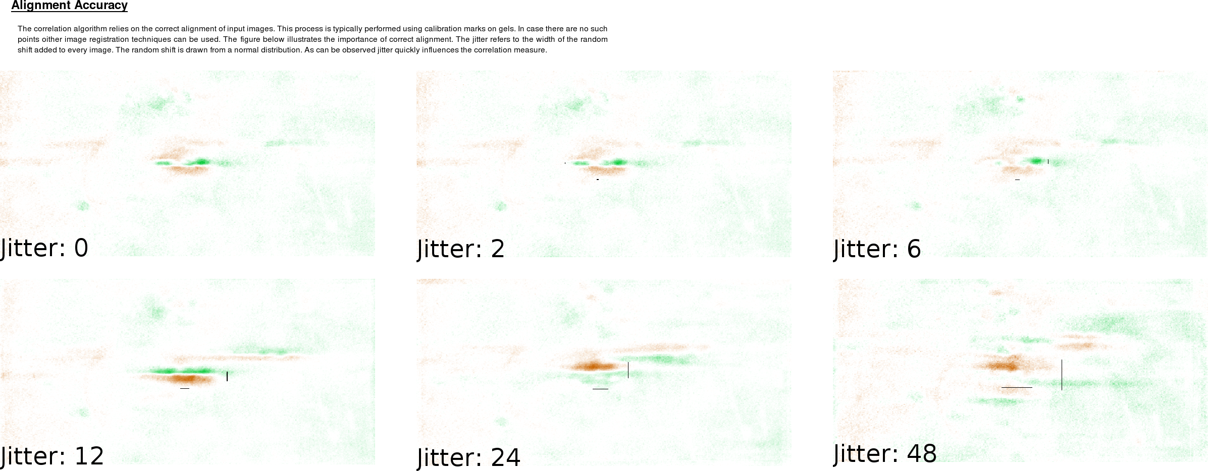
|
For this method to work properly, it is thus of great importance to rely on calibration spots and use these to register the images. Especially when working with large images that can contain many thousand spots, alignment is a known problem [44, 45]. Certain errors should be expected but as long as the spot jitter is smaller than the size of the spots, our algorithm will be able to provide useful results.
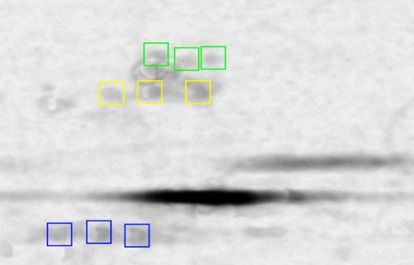
Intra-image correlations
A correlation measures indicates whether two data sets relate to each other, not how they relate. For instance, vectors [1,2,3] and [2,4,6] correlate with a value 1.0 without revealing the factor 2. As such, correlation should not be confused with up- or down-regulation, nor with a causal relationship. Nevertheless, if the correlation image reveals that one area goes down in pace with the external variable while another area goes up, it is natural to ask whether the relation between these two areas is of importance. Based on the FAB/p53 correlation, we will give two examples of such intra-image relations and explain how to address them at the pixel level.
Does the difference between p53- and p53-
 regions relate to the FAB classification ?
Fig. 4 reveals that the p53-![]() intensity increases
with higher differentiation while the p53-
intensity increases
with higher differentiation while the p53-![]() intensity decreases.
Therefore, we wondered whether the difference between p53-
intensity decreases.
Therefore, we wondered whether the difference between p53-![]() and p53-
and p53-![]() areas related
to the FAB classification. To answer
this question, we preprocessed the images to introduce the
'difference'.
This was achieved by summarizing the areas of interest and then
subtracting
those areas prior to correlation. Fig. 5
shows
the bounding boxes of the p53-
areas related
to the FAB classification. To answer
this question, we preprocessed the images to introduce the
'difference'.
This was achieved by summarizing the areas of interest and then
subtracting
those areas prior to correlation. Fig. 5
shows
the bounding boxes of the p53-![]() and p53-
and p53-![]() areas. Their
sizes, respectively
areas. Their
sizes, respectively ![]() and
and
![]() ,
were used to smooth the input images (and thus measure the total
intensity
within such areas). The shift between the area centers
,
were used to smooth the input images (and thus measure the total
intensity
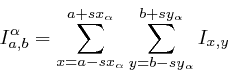
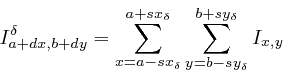
within such areas). The shift between the area centers ![]() was used to superimpose the
was used to superimpose the ![]() region over the
region over the ![]() region
prior to subtraction. If
region
prior to subtraction. If ![]() is
a 2DE image, then
is
a 2DE image, then ![]() and
and
![]() represented the two
intermediate images
represented the two
intermediate images
These two images were then subtracted to yield
![]() ,
which was subsequently put back into the gel-stack. If there was a
correlation between the
,
which was subsequently put back into the gel-stack. If there was a
correlation between the ![]() difference and the FAB classification
then we would find it at observation point
difference and the FAB classification
then we would find it at observation point ![]() in Fig. 5.
We did not find a correlation, indicating that the difference between
in Fig. 5.
We did not find a correlation, indicating that the difference between
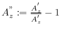
![]() -intensity and
-intensity and ![]() -intensity does not relate to the
FAB classification.
-intensity does not relate to the
FAB classification.
Does mass-difference relate to the FAB classification ?
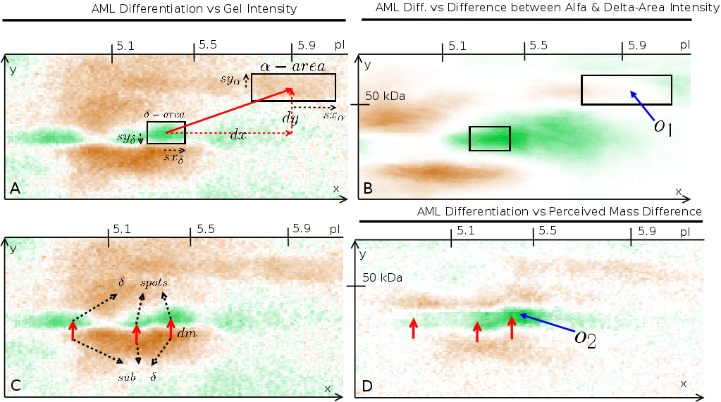 Figure 5: Intra-image testing for verification whether a combination
of opposing or similar correlations relates to the external variable.
When the correlation analysis reveals opposing or similar correlation
in two areas, the relation between those two areas might correlate
towards the external variable. Two examples are given. (A) shows that
the
Figure 5: Intra-image testing for verification whether a combination
of opposing or similar correlations relates to the external variable.
When the correlation analysis reveals opposing or similar correlation
in two areas, the relation between those two areas might correlate
towards the external variable. Two examples are given. (A) shows that
the |
Fig. 4 shows the sub-![]() region correlating negative
and the
region correlating negative
and the ![]() region
correlating positive, indicating that a mass-difference
might be related to the FAB classification. Setting up this specific
question is similar to the previous, but without summation of regions.
The image pre-processing measures the difference between the intensity
at a certain position
region
correlating positive, indicating that a mass-difference
might be related to the FAB classification. Setting up this specific
question is similar to the previous, but without summation of regions.
The image pre-processing measures the difference between the intensity
at a certain position ![]() and
intensities at the same position, but
with a lower mass (
and
intensities at the same position, but
with a lower mass (![]() ). If
). If ![]() is an image from the gel stack,
then
is an image from the gel stack,
then ![]() defines the new image
defines the new image
When using these preprocessed images into a correlation analysis,
we found that observation point ![]() revealed that indeed a mass-difference
relates to the FAB classification. Remembering the relative weak
correlation
in the FAB classification (0.2 and -0.2 at the specified areas), we
now find a much strong correlation: 0.507. This illustrates how the
correlation images can be used to naturally explore data sets.
revealed that indeed a mass-difference
relates to the FAB classification. Remembering the relative weak
correlation
in the FAB classification (0.2 and -0.2 at the specified areas), we
now find a much strong correlation: 0.507. This illustrates how the
correlation images can be used to naturally explore data sets.
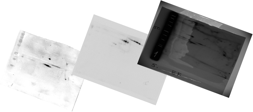
Spot shapes
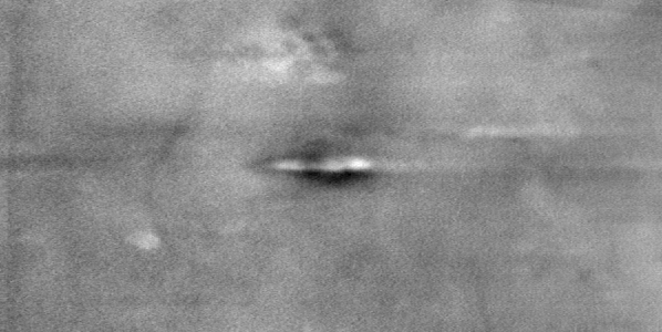
| ||||||
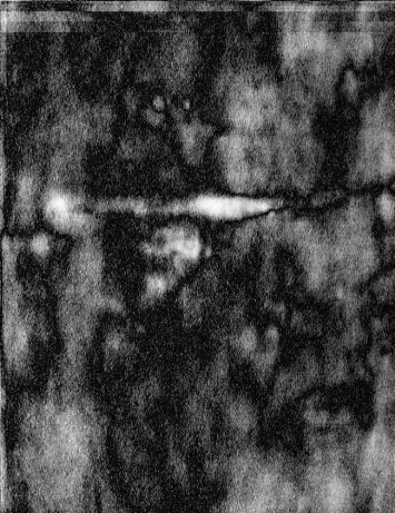
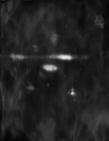
| Three images showing the difference in spot sizes between M0/M1/M2 and M4/M5 samples. The process of the changing spot distribution can be visualized by sorting all images according to their FAB classification and then showing them chronologically. This is visualized in a small movie. The two images and the movie are contained within a zip file. It can be extracted using unzip [46, 47]The movie can be played with mplayer [48] |
Performance
The complexity of the algorithm is linear to the size of the images
and the number of images. If we have ![]() images of width
images of width ![]() and
height
and
height ![]() then the calculation time
will be in the order of
then the calculation time
will be in the order of ![]() .
The
memory
considerations are the same because all images need to
be loaded in memory. E.g; 100 images of
.
The
memory
considerations are the same because all images need to
be loaded in memory. E.g; 100 images of
![]() pixels with
16 bit gray values will require around 200 Mb of internal memory.
More information on complexity measurement can be found at [49, 50].
pixels with
16 bit gray values will require around 200 Mb of internal memory.
More information on complexity measurement can be found at [49, 50].
Conclusions
The presented results demonstrated that the correlation method can provide valuable information about complexly regulated proteins in biological systems. The analysis technique can be used to measure and visualize relations between 2DE images and external (biological) variables. The correlation image is calculated based on an aligned stack of 2DE images. The resulting image can be naturally interpreted and offers information that might otherwise be unavailable (such as relevant changes in spot shape). The technique is robust, general applicable to different object types (tails, spots, areas), and allows a natural amount of spot location jitter. We also investigated calibration factors and it turned out that normalization factors barely influence the analytical power of the method.
The correlation analysis of p53 biosignatures on AML and ALL cancer
cells illustrated that the method can measure relations involving
the overall intensity of the biosignature. The novel findings of ALL-
and AML-specific p53 bioprofiles were verified on normal cells from
the lymphoid and myeloid lineages. The positive correlation for
full-length
and ![]() - p53 in ALL was reflected
by the presence of these p53
forms in lymphocytes, while these p53 forms were absent in the myeloid
granulocytes. This analysis of normal cells suggest that the
p53-distinction
between ALL and AML is correct.
- p53 in ALL was reflected
by the presence of these p53
forms in lymphocytes, while these p53 forms were absent in the myeloid
granulocytes. This analysis of normal cells suggest that the
p53-distinction
between ALL and AML is correct.
A second analysis illustrated that the correlation method differentiates between different protein isoforms. The relation between p53 biosignature and the AML FAB classification was more complex, which allowed us to explain how intra-image relations could answer specific questions. Doing so, we observed that a mass-difference in the p53 biosignature correlated strongly towards the FAB classification, suggesting that post-translational modifications of P53 relate to AML differentiation.
Future development of the method could include adjustments and corrections for hardware-parameters such as camera warping and different kinds of noise. Canonical correlations could be used to integrate information offered by similar neighboring correlation pixels [51, 52]. It could also be possible to insert clustering algorithms to pseudo-color the final image or use image segmentation algorithms to classify areas automatically [53, 54]. In its present form we believe the method provides a valuable tool to explore and analyze complex biosignatures and responses from signaling networks.
Methods
The correlation analysis
The 2DE image correlation technique relies on a large amount of 2DE
images of a biological system. Every gel needs to be described by
an external numerical measure. For every ![]() gels (described as
gels (described as ![]() in which
in which ![]() is the gel image number),
there are
is the gel image number),
there are ![]() external parameters,
described as
external parameters,
described as ![]() . Gels can
further be annotated as
. Gels can
further be annotated as ![]() in which
in which ![]() is the
position on gel number
is the
position on gel number ![]() .
. ![]() is
a vector containing the intensities of all gels:
is
a vector containing the intensities of all gels:
![]() .
.
Step 1: Alignment and registration
|
The method requires proper direction and alignment of all gels.
Presence
of calibration spots facilitates this process, otherwise techniques
such as Hough transformation [26, 55]for
gel direction measurement and cross correlation [56]for multiple gel alignment can be used. Once the gels are aligned,
further basic warping and registration [45]techniques
are
useful to account for small shifts between the different
gels. The aligned images are denoted ![]() .
.
Step 2: Intensity normalization
|
The second step normalizes the intensity values of the gels to allow for inter-gel pixel comparison. Currently, little known on the relation between pixel intensities and protein concentrations. The common assumption seems to center around linear scales. However, pixel values can be relative or gamma corrected, depending on the hardware. The wide variety of possible pixel value interpretations leads us to embrace the use of relative gray values. The simulated gel stack showed that the choice of normalization technique barely influences the final correlation image.
Step 2a: Background intensity
The background floor of a 2DE image refers to the brightness of empty
gel areas. Different capture techniques produce different background
floors. Background signal can be either added to all pixel values
(additive background), or it can accumulate with a decaying signal
(multiplicative background). As previously observed [44],
most
cameras
introduce a mixture of additive and multiplicative backgrounds.
Removal of additive noise can be done through subtracting the mean
(
![]() ) or median value (
) or median value (
![]() ).
Removal of multiplicative noise can be done through
).
Removal of multiplicative noise can be done through
 .
We would emphasize that whatever normalization scheme is used in this
step, it should be performed on an individual gel basis.
.
We would emphasize that whatever normalization scheme is used in this
step, it should be performed on an individual gel basis.
Step 2b: Scaling of gel intensity
After removal of the background floor, the dynamic range of the image
is normalized through scaling of gel intensities. The presence of
a calibration spot eases this process. If ![]() is the non-relative
image and
is the non-relative
image and ![]() is the
calibration spot position, then the image
is the
calibration spot position, then the image
 defines the normalized
image.
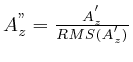
Without calibration spot the total energy content (sum of all
intensities
or RMS value) forms a very reasonable scaling means:
defines the normalized
image.
Without calibration spot the total energy content (sum of all
intensities
or RMS value) forms a very reasonable scaling means:
Step 3: Correlation image
|
|
After alignment and normalization, the correlation analysis generates
a new image visualizing the correlation measure between a specific
position and an external parameter. The correlation image is composed
of pixels, each testing one position on the gel. The result of each
test is a number between -1.0 (anti-correlation) and 1.0 (correlation),
which, after appropriate scaling, defines the pixel color in the
correlation
image. The two vectors participating in the test are ![]() and
and ![]() . The first vector
contains the gel expression levels at position
. The first vector
contains the gel expression levels at position
![]() . Given 89 gel images,
. Given 89 gel images, ![]() will contain 89 different
expression values; one for each gel. The second vector
will contain 89 different
expression values; one for each gel. The second vector ![]() contains
89 external values associated with every gel. Repeating this
correlation
test for every pixel results in the correlation image
contains
89 external values associated with every gel. Repeating this
correlation
test for every pixel results in the correlation image ![]() (Eq. 1)
(Eq. 1)
The correlation image can be visualized using different color schemes. In Fig. 1 green indicates positive correlations and brown negative correlations. Preferably one uses a hue scheme to avoid misinterpretation of correlation areas.
|
The preferred correlation is the robust Spearman rank order
correlation
(![]() -correlation)[27].
This
non-parametric test
allows us to ignore the specific distributions of gel intensity levels
and external parameters.
-correlation)[27].
This
non-parametric test
allows us to ignore the specific distributions of gel intensity levels
and external parameters. ![]() -correlation
requires
a ranking of
the two participating vectors and then relies on a standard linear
Pearson correlation. The ranking process will replace every value
in the input vector by its specific rank. When ties occur (the same
value occurring more than once) their rank will by convention be the
mean of their ranks as if they all would have had a slightly different
value.
-correlation
requires
a ranking of
the two participating vectors and then relies on a standard linear
Pearson correlation. The ranking process will replace every value
in the input vector by its specific rank. When ties occur (the same
value occurring more than once) their rank will by convention be the
mean of their ranks as if they all would have had a slightly different
value.
Step 4: Masking
| ||||||
Correlation does not necessarily imply a causal, significant, or useful relationship. To filter out some possibly useless relations, a number of masks limit the visible correlations. The first mask removes correlations that might be occurring by coincidence: some data sets easily correlate with any other data set (significance). The second mask removes correlations that offer little useful information (E.g: a data set containing all zero's).
Step 4a: Significance
To remove correlations that have a high probability of occurring, the significance test typically associated with the Spearman correlation test was used. In this context, it is defined as
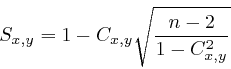
If this number is close to 1 then there exists a low probability that some random data would happen to correlate with the given result set. Likewise, if this number is 0 then there exists a high probability that the correlation is coincidental.
Step 4b: Variance
The second mask avoids strong and significant correlations that have a low biological significance because the gel intensities do not change enough. It relies on the standard deviation [57]measured on the relative, non-ranked, gel intensities
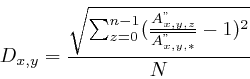
The standard variance (or RMS) of the mean divided gels will have a large value where there is a varying gel expression. At places where the gel expression is constant this value will be zero.
Step 4c: The masked correlation image
Multiplying the standard deviation mask (Eq. 3) with the significance mask (Eq. 2) gives a new mask that can be superimposed over the correlation image (Eq. 1).
The pixel values of ![]() no longer
relates to the correct correlation
measure. Therefore,
no longer
relates to the correct correlation
measure. Therefore, ![]() forms an
indicator, showing position of possible
interest.
forms an
indicator, showing position of possible
interest.
Step 5: Creating a correlation volume
|
Simulation of a 2DE image stack
The simulated gel-stack is based on the animation of different 2D Gaussian 'bumps', defined as
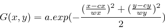
![]() is the center position,
is the center position, ![]() and
and ![]() are the width and
height respectively.
are the width and
height respectively. ![]() is the
amplitude of the curve. Based on
this Gaussian 'bump' a gel-stack, containing 15 different gels was
constructed. Every gel contains: I) an out-fading spot (Fig. 2,
spot
is the
amplitude of the curve. Based on
this Gaussian 'bump' a gel-stack, containing 15 different gels was
constructed. Every gel contains: I) an out-fading spot (Fig. 2,
spot ![]() ) with a
growing radius from
) with a
growing radius from ![]() to
to ![]() pixels
and lowering amplitude from
pixels
and lowering amplitude from ![]() to
to ![]() . II) An elliptical spot
(Fig. 2, spot
. II) An elliptical spot
(Fig. 2, spot ![]() ) which changes shape from being
small and tall
) which changes shape from being
small and tall ![]() to broad and
flat
to broad and
flat ![]() .
III) Two spots with minimal (1.0) and maximal (5.0) amplitudes (Fig.
2, spots
.
III) Two spots with minimal (1.0) and maximal (5.0) amplitudes (Fig.
2, spots ![]() ). IV) A moving spot (Fig. 2,
spot
). IV) A moving spot (Fig. 2,
spot
![]() ) from left to right.
) from left to right.
Patients
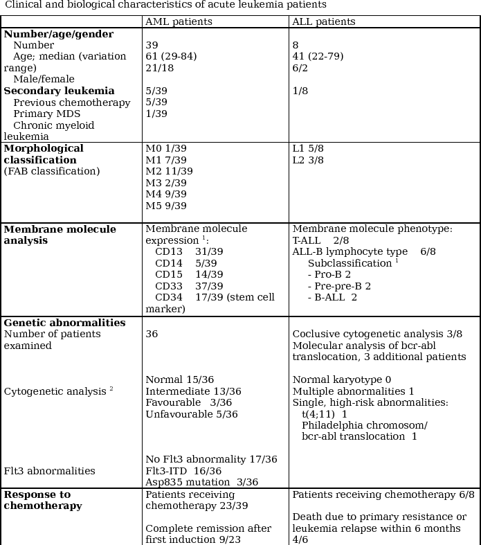 Table 1 - Clinical and biological characteristics of acute
leukemia patients Totally 73 AML and 16 ALL images were
included in the analysis. All ALL patients had B-cell disease and
two patients comprised the bcr-abl fusion
product.
Table 1 - Clinical and biological characteristics of acute
leukemia patients Totally 73 AML and 16 ALL images were
included in the analysis. All ALL patients had B-cell disease and
two patients comprised the bcr-abl fusion
product. |
The study was approved by the local Ethics Committee and samples
collected after informed consent. A total of 39 unique AML and 8 ALL patients
were analyzed by 2DE and immunoblotting for visualization of the p53
protein pattern by an amino-terminal targeting antibody Bp53-12.
Patients were immunophenotypically classified as positive when at least 20%
of the AML cells expressed the membrane molecule [58]. ALL
and AML was distinguished by immunophenotyping, see Table 1 with
characteristics.
AML FAB differentiation classification was determined by morphological
examination (microscopy) after May-Grunewald-Giemsa (MGG) staining
[37, 36], a
cytochemical stain that predominantly
reflects protein-features of the leukemia cells. Cytogenetic
abnormalities
in AML cells were classified according to Wheatley et al. [59].
The FAB classification is recently shown to be reflected in the gene
expression of the AML cells [38, 39]. The
AML patients
represent a consecutive group with high leukemia cell counts in
peripheral
blood (median blast count ![]() /L,
range
17-285), and at least
80% of the peripheral blood leukocytes were AML cells. The ALL patients
also represent a group of consecutive patients with high blood blast
counts (median
/L,
range
17-285), and at least
80% of the peripheral blood leukocytes were AML cells. The ALL patients
also represent a group of consecutive patients with high blood blast
counts (median ![]() /L,
range
49-560).
/L,
range
49-560).
Leukemic cell separation and sample preparation
Cell separation, storage and culture of patient AML blasts were performed as previously described [60, 28]. ALL and AML blasts were isolated by density gradient separation with Lymphoprep (Nycomed Pharma AS, Oslo, Norway) and contained more than 95% malignant cells. Normal granulocytes (97% neutrophile) and lymphocytes (peripheral blood mononuclear cells containing 10% monocytes and predominantly T lymphocytes) were separated by density gradient centrifuging combining Polymorphprep TM (Axis-Shield PoC AS, Oslo, Norway) and Lymphoprep following the manufacturers instructions. To avoid contamination of the myeloid monocytes in the lymphocytes, lymphocytes and monocytes were separated using an autoMACS magnetic sorter (Miltenyi Biotec GmbH). CD14+ cells (monocytes) were magnetically labelled with CD14 Microbeads (Miltenyi Biotec), following the procedure described by the manufacturer. CD14-PE antibody (Miltenyi Biotec) was used for flow cytometric determination of the purity of the two fractions (99% pure lymphocytes in flow through, 94% pure monocytes in magnetic eluate). Preparation for 2DE and immunoblotting was performed as previously described [61, 5, 62]. Briefly, cells were washed in NaCl (9 mg/ml) and then lysed in 7% trichloroacetic acid. The precipitated protein was washed once in 5% trichloroacetic acid and three times in water saturated ether to remove salts. The protein pellet was resuspended in sample buffer for 2DE gel electrophoresis (7 M urea, 2 M thiourea, 100 mM dithiotreitol, 1.5% Ampholyte 3 - 10, 0.5% Ampholyte 5 - 6, 0.5% CHAPS). 2D was performed using 7 cm pH 3-10 (Zoom Strip, Invitrogen Corp., Carlsbad, CA, USA) isoelectric focusing gel strips, following the manufacturers' instructions. Electrophoresis was performed at 200 V for 60 minutes, after which the proteins were transferred to polyvinylidene fluoride membrane (Amersham Biosciences AB, Uppsala, Sweden) by standard electro-blotting. p53 protein was detected using primary Bp53-12 antibody (Santa Cruz Biotechnology, CA, USA) and secondary horse radish peroxidase conjugated mouse antibody (Jackson ImmunoResearch, West Grove, PA, USA) visualized using the Supersignal West Pico or Femto Chemiluminescent Substrate system (Pierce Biotechnology, Inc., Rockford, IL, USA). Chemiluminescence imaging was performed using a Kodak Image Station 2000R (Eastman Kodak Company, Lake Avenue, Rochester, NY, USA) and were saved in TIFF format with the resolution of 300 DPI for correlation analysis.
Availability and requirements
The method can be freely used in academic environments. The source material given below includes correlation analysis, image coloring, Gaussian bumps and the simulated images. A user friendly version of the software was being developed at http://iis.yellowcouch.org/gelsignal-walkthrough.html
List of abbreviations
- [
 ]
Capital
letters are used to denote image matrices.
An image is an element of
]
Capital
letters are used to denote image matrices.
An image is an element of  .
.  and
and  are the width and height of the image.
 - [
 ]
Pixel
positions are written using subscript.
]
Pixel
positions are written using subscript.  refers to the gray value
of the pixel at position
refers to the gray value
of the pixel at position  in image
  . Subscripts are members
of
. Subscripts are members
of  .
. - [ALL] acute lymphoblastic leukemia
- [AML] acute myeloid leukemia
- [2DE] two-dimensional gel electrophoresis
- [FAB] The standardized French-American-British AML differentiation classification.
Author contributions
WVB invented and designed the correlation algorithm, processed the digitized images, designed and performed correlation analysis simulations, and drafted the manuscript. N� carried out the 2DE analysis of AML and ALL patient material, aligned the 2DE images and helped drafting the manuscript. IH designed and carried out PBMC analysis and helped to draft the manuscript. �B collected the AML biobank material, applied for ethical permission, collected clinical information and helped to draft the manuscript. BTG presented the original analysis challenge, helped to collect clinical data, coordinated the work and drafted the manuscript. All authors read and approved the final manuscript. WVB, N� and BTG contributed in the design of the study. KAH helped drafting the manuscript and contributed the idea to investigate the alignment accuracy.
Acknowledgments
Source
The source material includes correlation analysis,image coloring, Gaussian bumps and the simulated images.
The analysis method
d = size(all,/dim)
VX = d[1]
VY = d[2]
; normalize the background
for i = 0, d[0] - 1 do begin
all[i,*,*] /= mean(all[i,*,*])
endfor
; Rho correlation
cor_pic = make_array(VX,VY,/double,value=0.0)
f_pic = make_array(VX,VY,value=0.0)
for x = 0, VX - 1 do begin
for y = 0, VY - 1 do begin
r = r_correlate(reform(all[*,x,y]),result)
cor_pic[x,y]=r[0]
f_pic[x,y]=1.0-r[1]
endfor
endfor
; we are interested in correlations with high variance on gel
var_pic = make_array(VX,VY,/double,value=0.0)
for x = 0, VX - 1 do begin
for y = 0, VY - 1 do begin
var_pic[x,y]=stddev(all[*,x,y])
endfor
endfor
var_pic <= 1.0
f_pic *= var_pic
cor_pic <= 1.0
cor_pic >= -1.0
show_correlation, cor_pic, f_pic
end
Gauss Bumps
im = float(make_array(sx,sy,value=0.0))
for x = 0, sx - 1 do begin
for y = 0, sy - 1 do begin
im[x,y]=float(((cx-x)/wx)^2 + ((cy-y)/wy)^2)
endfor
endfor
im = -im/2
im = exp(im)
im *= a
return, im
end
Simulated Gel Stack
all = make_array(nr,sx,sy,value=0.0)
for i = 0, nr - 1 do begin
wx = wx1 + i*(wx2-wx1)/nr
wy = wy1 + i*(wy2-wy1)/nr
a = a1 + i*(a2-a1)/nr
all[i,*,*] = gauss2d(sx, sy, sx/2, sy/2, wx, wy, a)
endfor
return, all
end
set1 = create_set(15, 600.0, 400.0, 10.0, 100.0, 10.0, 100.0, 5.0, 1.0)
set2 = create_set(15, 300.0, 300.0, 10.0, 40.0, 40.0, 10.0, 5.0, 5.0)
set3 = create_set(15, 300.0, 300.0, 20.0, 20.0, 20.0, 20.0, 5.0, 5.0)
set4 = create_set(15, 300.0, 300.0, 20.0, 20.0, 20.0, 20.0, 1.0, 1.0)
set1[*,0:299,0:299] += set2[*,*,*]
set1[*,300:599,0:299] += set3[*,*,*]
set1[*,300:599,100:399] += set4[*,*,*]
for i = 0, 14 do begin
set1[i,0+i*10:299+i*10,200:399]+=set3[i,*,50:249]
endfor
for i = 0, 14 do begin
set1[i,*,*]/=double(i)
endfor
set1 = relative(set1)
result1 = findgen(15)
correlate_images, set1, result1
end
Creation of green/brown images
cor_pic = cp
DDD = size(cp,/dim)
VX = ddd[0]
VY = ddd[1]
; the normal one
shown = make_array(3,VX,VY,/double,value=255.0)
multi = 1.0 / max(abs(cor_pic))
multi = 1.0 / max(abs(cor_pic))
shown[0,*,*] += (cor_pic[*,*] < 0) * multi * 55
shown[1,*,*] += (cor_pic[*,*] < 0) * multi * 155
shown[2,*,*] += (cor_pic[*,*] < 0) * multi * 255
shown[0,*,*] -= (cor_pic[*,*] > 0) * multi * 255
shown[1,*,*] -= (cor_pic[*,*] > 0) * multi * 55
shown[2,*,*] -= (cor_pic[*,*] > 0) * multi * 205
window, 1, title='Correlation', ret=2, xsize=vx, ysize=vy
shown >= 0
shown <= 255
tvscl, shown, /true
; only the significant correlation
wcor_pic = double(cor_pic) * double(t_pic)
shown = make_array(3,VX,VY,/double,value=255.0)
multi = 255.0 / max(abs(wcor_pic))
shown[0,*,*] += (wcor_pic[*,*] < 0) * multi * 55
shown[1,*,*] += (wcor_pic[*,*] < 0) * multi * 155
shown[2,*,*] += (wcor_pic[*,*] < 0) * multi * 255
shown[0,*,*] -= (wcor_pic[*,*] > 0) * multi * 255
shown[1,*,*] -= (wcor_pic[*,*] > 0) * multi * 55
shown[2,*,*] -= (wcor_pic[*,*] > 0) * multi * 205
window, 3, title='Significant Correlations', ret=2, xsize=vx, ysize=vy
tvscl, shown, /true
shown = bytscl(shown)
profiles, cor_pic
; significance
window, 2, title='Significance', ret=2, xsize=vx, ysize=vy
tvscl, t_pic
profiles, t_pic
end
Bibliography
| 1. | High Resolution two-dimensional electrophoresis of proteins P. H. O'Farrell J. Biol. Chem.; volume: 250; number: 10; pages: 4007-21; May 25; 1975 |
| 2. | Current two-dimensional electrophoresis technology for proteomics. A. Gorg, W. Weiss, M.J. Dunn Proteomics; volume: 4; number: 12; pages: 3665-3685; Dec; 2004 |
| 3. | Identification of extracellular and intracellular signaling components of the mammary adipose tissue and its interstitial fluid in high risk breast cancer patients: toward dissecting the molecular circuitry of epithelial-adipocyte stromal cell interactions J.E. Celis, J.M. Moreira, T. Cabezon, P. Gromob, R. Friis, F. Rank, I. Gromova Mol Cell Proteomics; volume: 4; number: 4; pages: 492-522; February; 2005 |
| 4. | Proteomic Analysis of the cell-surface membrane in chronic lymphocytic leukemia: identification of two novel proteins, BCNP1 and MIG2B R.S. Boyd, P.J. Adams, S. Patel, J.A. Loader, J. Berry, N.T. Redpath, H.R. Poyser, G.C. Fletcher, N.A. Burgess, A.C. Stamps, L. Hudson, P. Smith, M. Griffiths, T.G. Willis, E.L. Karran, Oscier D.G., D. Catovsky, J.A. Terrett, M.J. Dyer Leukemia; volume: 17; number: 8; pages: 1605-1612; 2003 |
| 5. | Analysis of acute myelogenous leukemia: preparation of samples for genomic and proteomic analysis Bjørn Tore Gjertsen, A.M. Oyan, B. Marzolf, Randi Hovland, G. Gausdal, Stein Ove Doskeland, K. Dimitrov, A. Golden, K.H. Kalland, L. Hood, Ø. Bruserud J Hematother Stem Cell Res; volume: 11; number: 3; pages: 469-81; June; 2002 |
| 6. | Proteomics in acute myelogenous leukemia (AML): methodological strategies and identification of protein targets for novel antileukemic therapy. Gry Sjoholt, Nina Ånensen, L Wergeland, E McCormak, Ø Bruserud, Bjørn Tore Gjertsen Current Drug Targets; volume: 6; number: 6; pages: 631-646; 2005 |
| 7. | Acute myeloid and T-cell acute lymphoblastic leukaemia with aberrant antigen expression exhibit similar TCRdelta gene rearrangements. C.A. Schmidt, G. Przybylski, A. Tietze, H. Oettle, W. Siegert, W.D. Ludwig Br. J. Haematol; volume: 92; number: 4; pages: 929-36; 1996 |
| 8. | Disease proteomics. S. Hanash Nature; volume: 422; number: 6928; pages: 226-32; 2003 |
| 9. | Cancer diagnosis using proteomic patterns. T.P. Conrads, M. Zhou, E.F. Petricoin, L. Liotta, T.D. Veenstra Expert Rev Mol Diagn; volume: 3; number: 4; pages: 411-20; 2003 |
| 10. | Proteomic analysis of human acute leukemia cells: insight into their classification J.W. Cui, J. Wang, K. He, B.F. Jin, H.X. Wang, W. Li, L.H. Kang, M.R Hu, H.Y. Li, M. Yu, B.F. Shen, G.J. Wang, X.M. Zang Clin Cancer Res; volume: 10; number: 20; pages: 6887-96; October; 2004 |
| 11. | Two-dimensional gel electrophoresis and computer analysis of proteins synthesized by clonal cell lines. J.I. Garell J. Biol. Chem.; volume: 254; number: 16; pages: 7961-7977; 1979 |
| 12. | Advances in two-dimensional gel matching technology S. Curch Biochem Soc Trans; volume: 32; number: Pt3; pages: 511-516; June; 2004 |
| 13. | Computer-analyzed high resolution two-dimensional gel electrophoresis: a new window for protein research S.H. Blose, S.A. Hamburger Biotechniques; volume: 3; pages: 232-236; 1985 |
| 14. | Uses of digital image analysis in electrophoresis Horgan, G.W., Glasbey, C. A. Electrophoresis; volume: 16; pages: 298-305; March; 1995 |
| 15. | The MELANIE Project: from a biopsy to automatic protein map interpretation by computer Appel, R., Hochstrasser, D.F., Funk, M., Vargas, J.R., Pellegrini, C., Muller, A.F., Sherrer, J.R. Electrophoresis; volume: 12; pages: 722-735; 1991 |
| 16. | Analyzing Two-Dimensional Gel Images Roy Anindya, R. Lee Kwan, Hang Yaming, Mark Marten, Raman Babu institution: Department of Mathematics and Statistics, University of Maryland; August; 2003 |
| 17. | Towards validating a method for two-dimensional electrophoresis/silver staining Wolfgang Schlags, Michael Walther, Mohammed Masree, Martin Kratzel, Christian R. Noe, Bodo Lachmann Electrophoresis; volume: 26; pages: 2461-2469; 2005 |
| 18. | The importance of diagnostic cytogenetics on outcome in AML: analysis of 1612 patients entered into the MRC AML 10 trial. D. Grimwade, H. Walker, F. Oliver, K. Wheatley, C. Harrison, J. Rees, I. Hann, R. Stevens, A. Burnett, A. Goldstone The Medical Research Council Adult and Children's Leukaemia Working Parties; Blood; volume: 92; pages: 2322-33; 1998 |
| 19. | The Molecular Basis of Leukemia D.G. Gilliland, C.T. Jordan CT, C.A. Felix Hematology (Am. Soc. Hematol. Educ. Program); pages: 80-97; 2004 |
| 20. | Targeting mutated protein tyrosine kinases and their signaling pathways in hematologic malignancies Y. Chaladon, J. Schwaller Haematologica; volume: 90; pages: 949-68; 2005 |
| 21. | Genes causing inherited cancer as beacons to identify the mechanisms of chemoresistance P.E. Lonning Trends Mol. Med.; volume: 10; number: 3; pages: 113-118; Mar; 2004 |
| 22. | Post-translational modifications of p53 in tumorigenesis A.M. Bode, Z. Dong Nat. Rev. Cancer; volume: 4; number: 10; pages: 793-805; Oct; 2004 |
| 23. | The p53 pathway: positive and negative feedback loops S.L. Harris, A.J. Levine Oncogene; volume: 24; number: 17; pages: 2899-908; 18 April; 2005 |
| 24. | Protein p53 and inducer-mediated erythroleukemia cell commitment to terminal cell division D.W. Shen, F.X. Real, A.B. DeLeo, L.J. Old, P.A. Marks, R.A. Rifkind Proc Natl Aca Sci USA; volume: 80; number: 19; pages: 5919-22; October; 1983 |
| 25. | Wt-p53 action in human leukemia cell lines corresponding to different stages of differentiation MG Rizzo, A. Zepparoni, B. Cristofanelli, R. Scardigli, M. Crescenzi, G. Blandino, S. Giuliacci, S. Ferrari, S. Soddu, A. Sacchi Br J Cancer; volume: 77; number: 9; pages: 1429-1438; May; 1998 |
| 26. | Digital Image Processing Rafael C. Gonzalez, Richard E. Woods Prentice Hall; chapter: 7; pages: 432-438; address: Upper Saddle River, New Jersey 07458; edition: 2nd; 2002 |
| 27. | Numerical Recipes in C++ William T. Veterling, Brian P. Flannery Cambridge University Press; editor: William H. Press and Saul A. Teukolsky; chapter: 10; edition: 2nd; February; 2002 |
| 28. | Single Cell profiling of potentiated phospho-protein networks in cancer cells J.M. Irish, R. Hovland, P.O. Krutzik, O.D. Perez, Ø. Bruserud, B.T. Gjertsen, G.P. Nolan Cell; volume: 118; pages: 217-228; 2004 |
| 29. | Intracellular signal transduction pathway proteins as targets for cancer therapy AA Adjei, M. Hidalgo J Clin Oncol; volume: 10; number: 23; pages: 5386-403; Aug; 2005 |
| 30. | p53 isoforms can regulate p53 transcriptional activity J.C. Bourdon, K. Fernandes, F. Murray-Zmijewski, G. Liu, A. Diot, D.P. Xirodimas, M.K. Saville, D.P. Lane Genes Dev; volume: 19; number: 18; pages: 2122-37; Sep 15; 2005 |
| 31. | Multisite phosphorylation and the integration of stress signals at p53 DW Meek Cell Signal; volume: 10; number: 3; pages: 159-66; Mar; 1998 |
| 32. | Acute myeloid leukemia RM Stone, MR O'Donnell, MA Sekeres Hematology (Am Soc Hematol Educ Program); pages: 98-117; 2004 |
| 33. | Acute lymphoblastic leukemia D. Hoelzer, N. Gokbuget, O. Ottmann, CH Pui, MV Relling, FR Appelbaum, JJ van Dongen, T. Szczepanski Hematology (Am Soc Hematol Educ Program); pages: 162-92; 2002 |
| 34. | Growth factor receptor profile of CD34+ cells in AML and B-lineage ALL and in their normal bone marrow counterparts. M De Waele, W. Renmans, K. Vander Gucht, K. Jochmans, R. Schots, J. Otten, F. Trullemans, P. Lacor, I. Van Riet Eur J Haematol; volume: 66; number: 3; pages: 178-87; Mar; 2001 |
| 35. | Routine expression profiling of microarray gene signatures in acute leukaemia by real-time PCR of human bone marrow E. Sakhinia, M. Faranghpour, JA Liu Yin, G. Brady, JA Hoyland, RJ Byers. Br J Haematol; volume: 130; number: 2; pages: 233-48; Jul; 2005 |
| 36. | Proposal for the recognition of minimally differentiated acute myeloid leukemia (AML-M0). J.M. Bennett, D. Catovsky, M.T. Daniel, G. Flandrin, D.A. Galton, H.R. Gralnick, C. Sultan Br J Haematol; volume: 78; pages: 325-329; 1991 |
| 37. | Proposals for the classification of the acute leukaemias. French-American-British (FAB) co-operative group. J.M. Bennett, D. Catovsky, M.T. Daniel, G. Flandrin, D.A. Galton, H.R. Gralnick, C. Sultan Br J Haematol; volume: 33; pages: 451-458; 1976 |
| 38. | Use of gene-expression profiling to identify prognostic subclasses in adult acute myeloid leukemia. L. Bullinger, K. Dohner, E. Beir, S. Frohling, R.F. Schlenk, R. Tibshirani, H. Dohner, J.R. Pollack N Engl J Med; volume: 16; number: 350; pages: 1605-16; April 15; 2004 |
| 39. | Prognostically useful gene-expression profiles in acute myeloid leukemia. P.J. Valk, R.G. Verhaak, M.A. Beijen, C.A. Erpelinck, Barjesteh van Waalwijk van Doorn- S. Khosrovani, J.M. Boer, H.B. Beverloo, M.J. Moorhouse, P.J. van der Spek, B. Lowenberg, R. Delwel N Engl J Med; volume: 16; number: 350; pages: 1617-28; April 15; 2004 |
| 40. | Wild-type p53 gene expression induces granulocytic differentiation of HL-60 cells S. Soddu, G. Blandino, G. Citro, R. Scardigli, G. Piaggio, A. Ferber, B. Calabretta, A. Sacchi Blood; volume: 83; number: 8; pages: 2230-7; April 15; 1994 |
| 41. | Induction of IW32 erythroleukemia cell differentiation by p53 is dependent on protein tyrosine phosphatase P.P. Tang, F.F. Wang Leukemia; volume: 14; pages: 1292-1300; 2000 |
| 42. | p53 induces differentiation of mouse embryonic stem cells by suppressing Nanog expression T. Lin, C. Chao, S. Saito, S.J. Mazur, M.E. Murphy, E. Apella, Y. Xu Nat Cell Biol.; volume: 7; number: 2; pages: 165-171; February; 2005 |
| 43. | 1999 World Health Organization Classification of Neoplastic Diseases of the Hematopietic and Lymphoid Tissues: report on the Clinical Advisory Committee Meeting, Arlie House, Virginia NL Harris, ES Jaffe, J Diebold, G. Flandrin, HK Muller-Hermelink, J. Vardiman, TA Lister, CD Bloomfield J. Clin Oncol; volume: 17; pages: 3835-384; November; 1997 |
| 44. | Adaptive Contrast Enhancement of Two-Dimensional Electrophoretic Gels Facilitates Visualization, Orientation and Alignment Werner Van Belle, Gry Sjøholt, Nina Ånensen, Kjell-Arild Høgda, Bjørn Tore Gjertsen Electrophoresis; Wiley Interscience Vch; volume 27; nr 20; pages 4086-4095; October 2006 http://werner.yellowcouch.org/Papers/2ddenois/index.html |
| 45. | Hybrid Registration for Two-Dimensional Gel Protein Images Xiuying Wang, David Dagan Feng Third Asia Pacific Bioinformatics Conference (APBC2005); January; 2005 |
| 46. | Winzip - The ZIP Utility for windows http://www.winzip.com/ |
| 47. | ZipIt: Macintosh Compression Utility http://www.maczipit.com/ |
| 48. | Mplayer Headquarters http://www.mplayerhq.hu/ |
| 49. | Big O Notation http://en.wikipedia.org/wiki/Big_O_notation |
| 50. | The Art of Computer Programming Donald Knuth Addison-Wesley; chapter: 1.2.11: Asymptotic Representations; pages: 107-123; volume: 1; edition: 3th; 1997 |
| 51. | Robust Canonical Correlations: A Comparative Study J.A. Branco, C. Croux, P. Filzmoser, M.R. Oliviera Computational Statistics; volume: 20; pages: 203-229; 2005 |
| 52. | Data Analysis, Classification, and Related Methods C. Dehon, P. Filzmoser, C. Croux H.A.L. Kiers and J.P. Rasson and P.J.F. Groenen and M. Schrader; editor: Berlin: Springer-Verlag; chapter: Robust Methods for Canonical Correlation Analysis; pages: 321-326; 2000 |
| 53. | Maximum Entropy and Bayesian Methods J. Stutz and P. Cheeseman Cambridge 1994; chapter AutoClass - a Bayesian Approach to Classification. Kluwer Acedemic Publishers, Dordrecht, 1995. |
| 54. | Advances in Knowledge Discovery and Data Mining P. Cheeseman and J. Stutz chapter Bayesian Classification (AutoClass): Theory and Results. AAAI Press/MIT Press, 1996. |
| 55. | Methods and Means for Recognizing Complex Patterns Hough, P.V.C US Patent 3,069,654; 1962 |
| 56. | Analysis of two-dimensional electrophoresis gels K. Conradsen, J. Pedersen Biometrics; volume: 48; pages: 1273-1287; 1992 |
| 57. | The Standard Deviation and Calculation of the Standard Deviation J.F. Kenny, E.S. Keeping Princeton NJ; editor: Van Nostrand; chapter: 6.5--6.6; pages: 77-80; edition: 3th; 1962 |
| 58. | Proposals for the immunological classification of acute leukemias. European Group for the Immunological Characterization of Leukemias (EGIL). M.C. Bene, G. Catoldi, W. Knapp, W.D. Ludwig, E. Matutes, A. Orfao, M.B. Van't Veer Leukemia; volume: 9; number: 10; pages: 1783-6; Oct; 1995 |
| 59. | A simple, robust, validated and highly predictive index for the determination of risk-directed therapy in acute myeloid leukaemia derived from the MRC AML 10 trial. United Kingdom Medical Research Council's Adult and Childhood Leukaemia Working Parties K. Wheatley, A.K. Burnett, A.H. Goldstone, R.G. Gray, I.M. Hann, C.J. Harrison, J.K. Rees, R.F. Stevens, H. Walker Br J Haematol.; volume: 107; number: 1; pages: 69-79; October; 1999 |
| 60. | Flt3-mediated signaling in human acute myelogenous leukemia (AML) blasts: a functional characterization of Flt3-ligand effects in AML cell populations with and without genetic Flt3 abnormalities Øystein Bruserud, Randi Hovland, L. Wergeland, T.S. Huang, Bjørn Tore Gjertsen Haematologica; volume: 88; pages: 416-428; 2003 |
| 61. | Characterization of ribosomal P autoantibodies in relation to cell destruction and autoimmune disease. E. Ersvaer, L.T. Bertelsen, L.C. Espenes, T. Bredholt, S.O. Boe, B.M. Iversen, Øystein Bruserud, E. Ulvestad, Bjørn Tore Gjertsen Scan J Immunol; volume: 60; number: 2; pages: 189-198; Aug; 2004 |
| 62. | Novel (Rp)-cAMPS analogs as tools for inhibition of cAMP-kinase in cell culture. Basal cAMP-kinase activity modulates interleukin-1-beta action B. T. Gjertsen, G. Mellgren, A. Otten, E. Maronde, H. G. Genieser, B. Jastroff, O.K. Vintermyr, G. S. McKnight, S. O. Doskeland J Biol Chem; volume: 270; number: 35; pages: 20599-607; Sep 1; 1995 |
| http://werner.yellowcouch.org/ werner@yellowcouch.org |  |