| Home | Papers | Reports | Projects | Code Fragments | Dissertations | Presentations | Posters | Proposals | Lectures given | Course notes |
|
|
Beatgraphs: Music at a GlanceWerner Van Belle1 - werner@yellowcouch.org, werner.van.belle@gmail.com Abstract : Explained are beatgraphs, a music visualisation technique that allows one to see rhythmical patterns, recognize frequencies and observer the musical structure in the blink of an eye.
Keywords:
beatgraphs, carpet plot, music visualisation |
Table Of Contents
Introduction
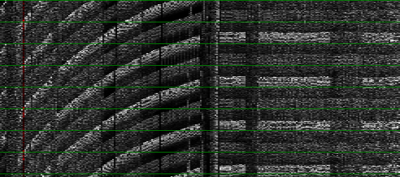
A 'Beatgraph' is a way to visualize music, that was originally introduced in BpmDj [1, 2, 3]. It requires knowledge of the length of 1 bar and the start of the first beat in that bar. Based on that information the music energy is then shown from top to bottom, and left to right. Each pixel-column visualizes the content of 1 bar. Below is a demonstration of such a beatgraph.
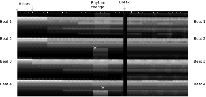 A black/white beatgraph. From left
to right musical bars are visualized. From top to bottom the energy
content of each bar. Bright pixels ~ much energy, dark pixels
~ little energy
A black/white beatgraph. From left
to right musical bars are visualized. From top to bottom the energy
content of each bar. Bright pixels ~ much energy, dark pixels
~ little energy
|
The above picture shows the pattern visualization of a simply 4/4 drum loop. Although at first it looks confusing it does show the entire song in one picture. 4 broad horizontal bands catch the eye. Each band represents a beat.
Some features of beatgraphs
- A beatgraph shows us how many beats we have per bar. In this case 4. In a 3/4 rhythm we would only see 3 beats per bar (i.e. three horizontal lines)
- A beatgraph shows the full energy content of a song, includingat which positions breaks (no energy) and buildups (gradually increasing brightness) occur.
- A beatgraph gives us an overall sense of the rhythm (we have a beat positioned at each 4th note) and can tell us at what position rhythm changes occur. This can even be formalized into a rhythm extraction algorithm as given by [4]
- A beatgraph provides an overall sense of composition. E.g: a change occurs every 4, 8 or 16 bars.
- It tells us whether the rhythm spans 1 or 2 bars. In case the rhythm repeats every two bars (as opposed to every bar), one sees a distinct interleaving between the various pixel columns.
- It tells us whether the tempo is steady or floating, and if it is floating where and how.
- Lastly a beatgraph tells us the location of the first beat in a bar by always positioning the start of a bar at the top of the image.
| ||||
| Some demos of non ordinary rhythms |
Energy visualisations
In this section I describe various approaches to visualize the songs' energy-content. The goal is of course to pack as much useful information in each pixel as possible.... without overcrowding it.
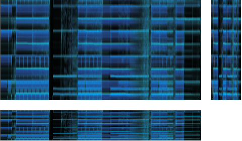
Amplitudes
| ||||
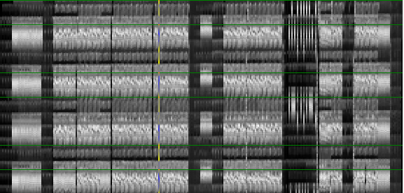
| Amplitude beatgraphs |
The first beatgraph (made in 2001) simply sampled the absolute value of the audio amplitude. That was directly mapped to the pixel intensity.
In the above image we see two songs with a floating tempo. In the left one, the drummer has no sense of time and apparently just hits the bass drum whenever he feels like it. In the right one, the tempo change is gradually (probably a down spinning turntable as to match the tempo of the new song). As soon as the new song kicks in the tempo is steady.
The use of absolute values led to very interesting interference patterns, but was somewhat too unstable: every time we drew the beatgraph using a different height for the image, we would see totally different interferences. Aside from this drawback, they are also somewhat visually unappealing.
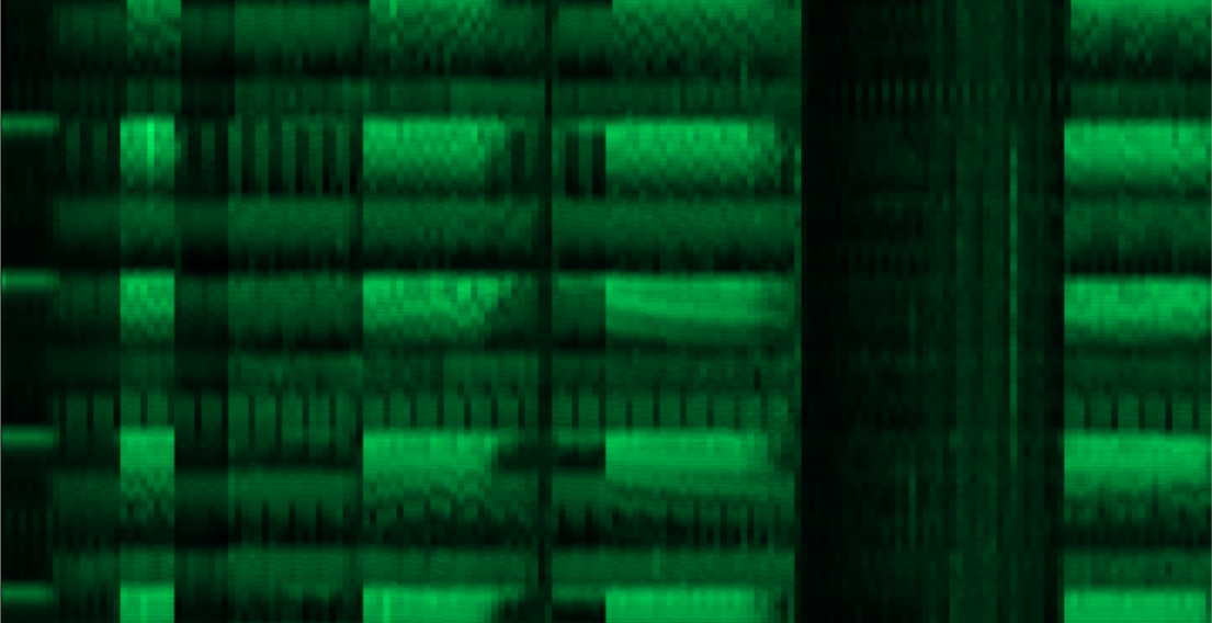
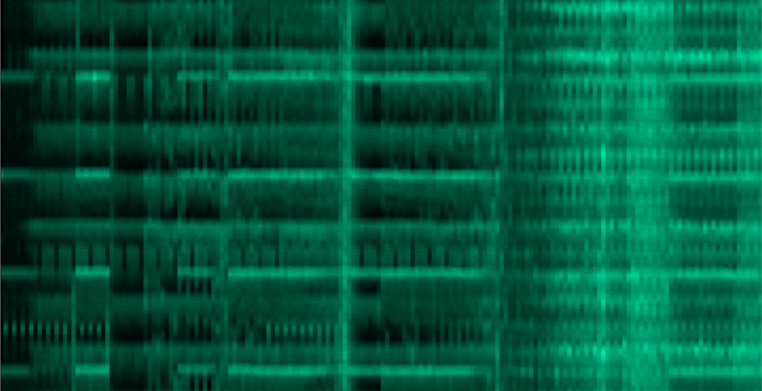
RMS
| ||||
| RMS Beatgraph |
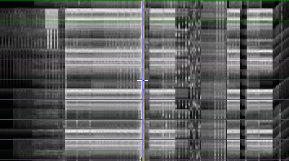
An approach that reduces the interference patterns, is to use RMS values (created in 2006) of the audio spanned by each pixel. This is very suitable to create monochrome pictures. The problem is however that certain tracks have a constant energy throughout the entire track, which washes away the brightness of the transients. This can be solved as we will discuss later.
One could also experiment with a logarithmic interpretation (dB measure as opposed to RMS). That is however a moot point since, at a later stage one must often fiddle with the gamma correction of the image to bring out the transients correctly.
Wavelets
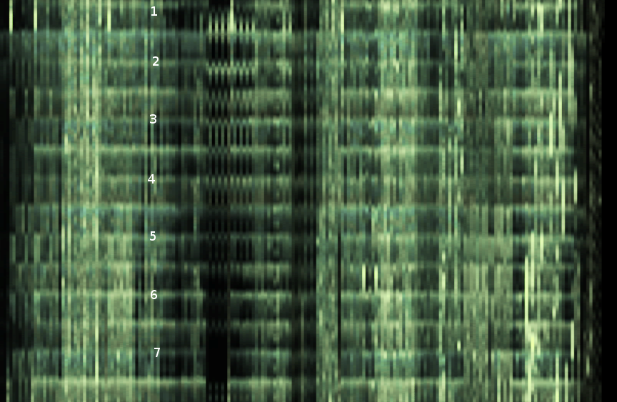
One approach to bring some order in all those gray pixels is to split the frequency bands and assign different colors to different frequency bands.
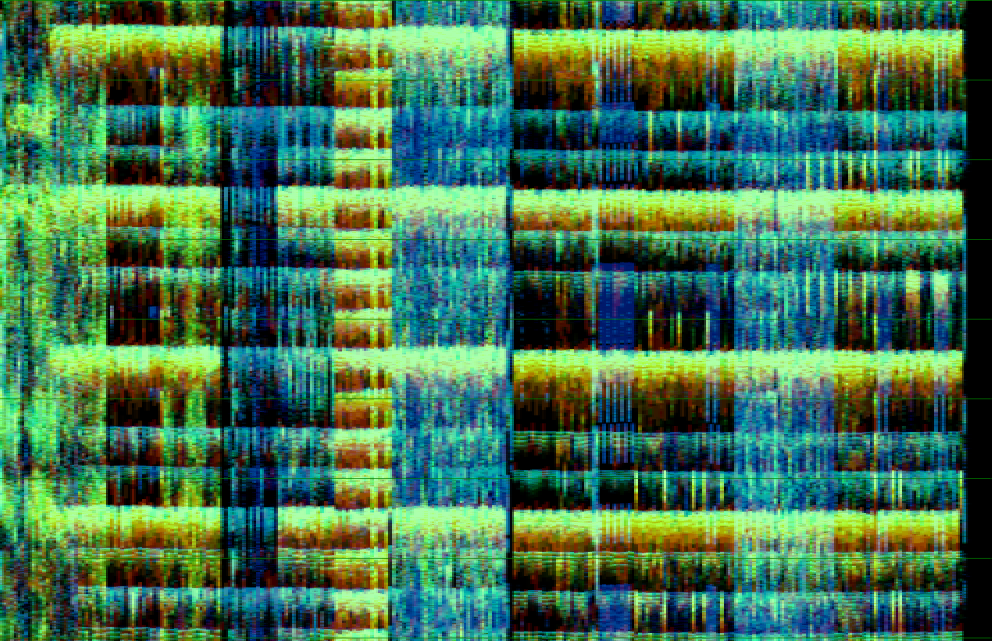 Wavelet based
beatgraph (10 haar bands). Red over yellow to blue spans the spectrum
from lo to high frequencies.
Wavelet based
beatgraph (10 haar bands). Red over yellow to blue spans the spectrum
from lo to high frequencies.
|
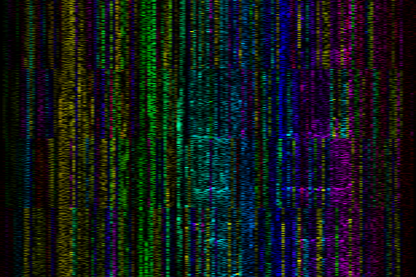
This technique (first implemented in 2003) splits the signal in multiple bands and then decides on the hue based on the presence of the different frequencies. In this case a Haar [5] wavelet was used, which resulted in the following band boundaries
- 43.066406 Hz
- 86.132812 Hz
- 172.26562 Hz
- 344.53125 Hz
- 689.0625 Hz
- 1378.125 Hz
- 2756.25 Hz
- 5512.5 Hz
- 11025 Hz
- 22050 Hz
- 44100 Hz
A drawback of using 10 frequency bands, is that we somehow need to map those 10 bands to a color. This can be done by assigning to each band a specific hue and then adding all those colors together. The result is not very satisfying: we often only see 2 or at most 3 pieces of information (in the above picture one cannot easily figure out where the middle frequencies are). A second problem is that high frequencies are available at a fairly high samplerate, again producing interference patterns. That can be solved by either measuring the energy over larger time windows, by adding an amplitude decay over 200 milliseconds, or by applying different filters.
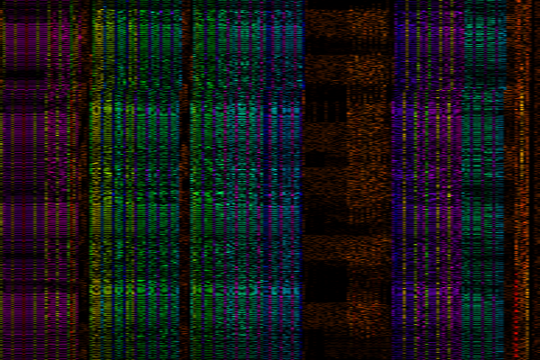
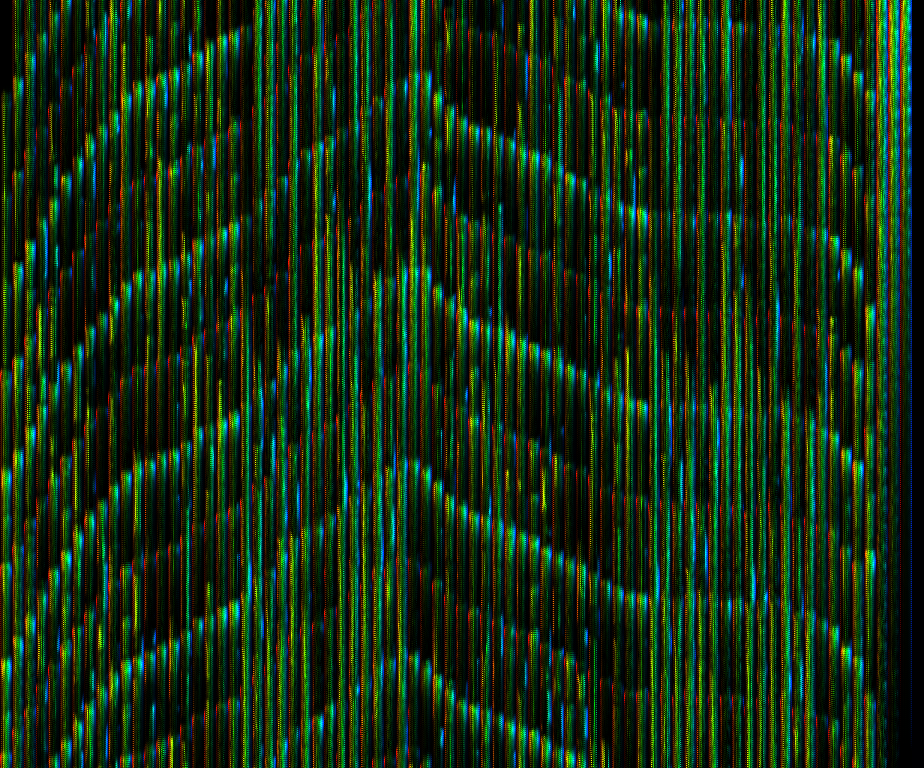
Critical bands
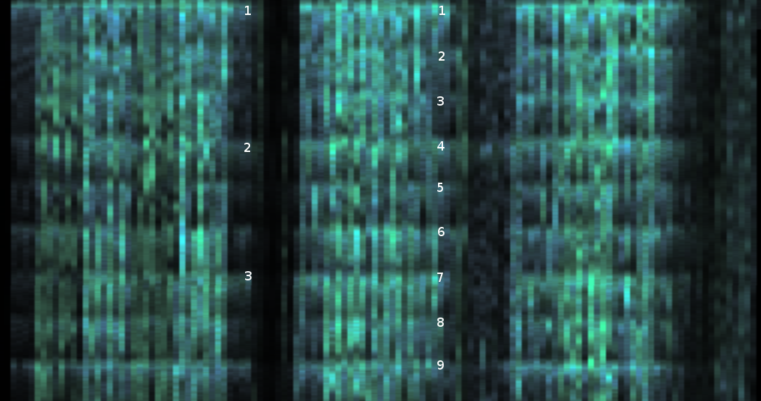
Another possibility to map multiple bands to a single color, is to rely on a grid in which we color each subpixel appropriately (2010). For instance, if we have 24 frequency bands then we could use 24 subpixels per pixel. Each subpixel would be as intense as the energy in that band. Below is a zoom in of such a visualization grid. The full images are given below.
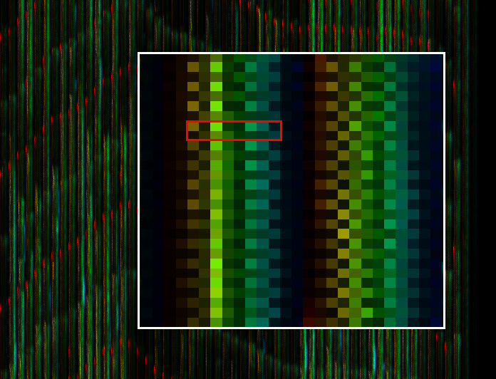 The visualisation grid. Each cell
is 12 subpixels wide and 2 subpixels high. The red box contains one 'pixel'.
The visualisation grid. Each cell
is 12 subpixels wide and 2 subpixels high. The red box contains one 'pixel'.
|
| ||||
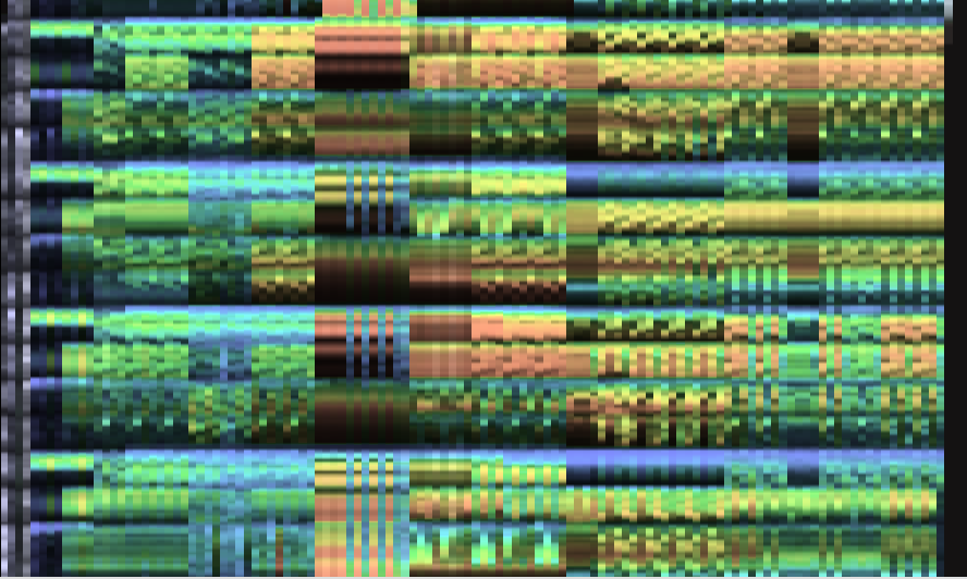
| Spectral beatgraph based on critical bands and regular dithering |
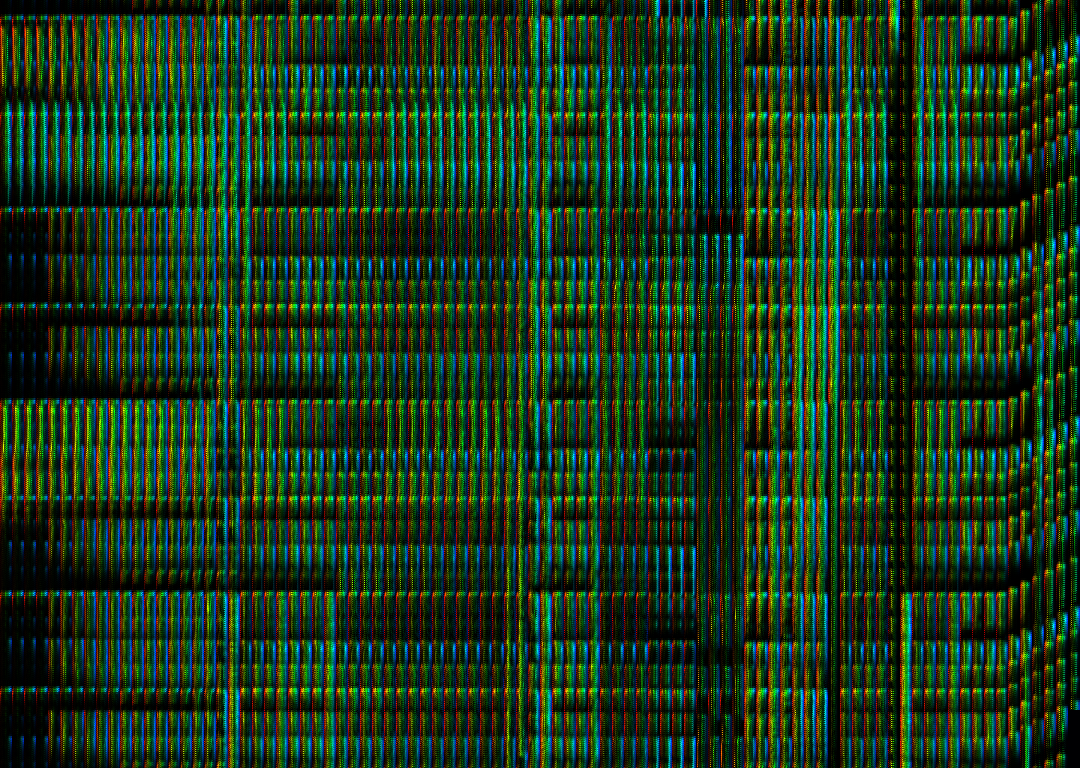
The 24 frequency bands used are the 24 critical bands of hearing; also called the Bark frequency bands [6]
- Bark 1 from 0 Hz to 100 Hz.
- Bark 2 from 100 Hz to 200 Hz.
- Bark 3 from 200 Hz to 300 Hz.
- Bark 4 from 300 Hz to 400 Hz.
- Bark 5 from 400 Hz to 510 Hz.
- Bark 6 from 510 Hz to 630 Hz.
- Bark 7 from 630 Hz to 770 Hz.
- Bark 8 from 770 Hz to 920 Hz.
- Bark 9 from 920 Hz to 1080 Hz.
- Bark 10 from 1080 Hz to 1270 Hz.
- Bark 11 from 1270 Hz to 1480 Hz.
- Bark 12 from 1480 Hz to 1720 Hz.
- Bark 13 from 1720 Hz to 2000 Hz.
- Bark 14 from 2000 Hz to 2380 Hz.
- Bark 15 from 2380 Hz to 2700 Hz.
- Bark 16 from 2700 Hz to 3150 Hz.
- Bark 17 from 3150 Hz to 3700 Hz.
- Bark 18 from 3700 Hz to 4400 Hz.
- Bark 19 from 4400 Hz to 5300 Hz.
- Bark 20 from 5300 Hz to 6400 Hz.
- Bark 21 from 6400 Hz to 7700 Hz.
- Bark 22 from 7700 Hz to 9500 Hz.
- Bark 23 from 9500 Hz to 12000 Hz.
- Bark 24 from 12000 Hz to 15500 Hz.
Although as appealing as this approach might be, the resolution of the display must be large. E.g: when a song has 100 bars, one needs already 1200 pixels, which is often too much.
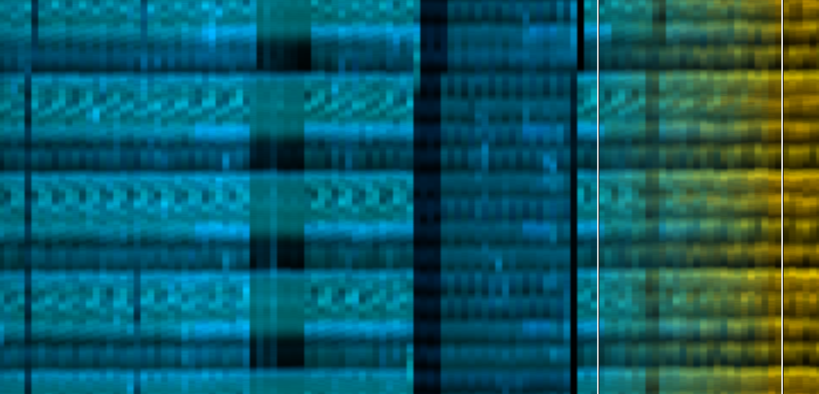
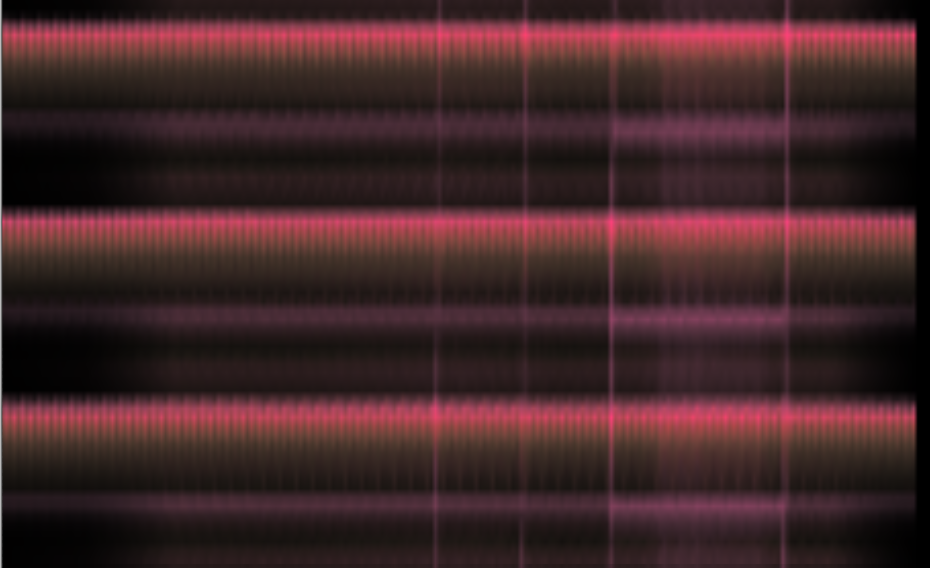
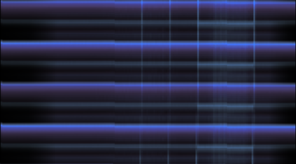
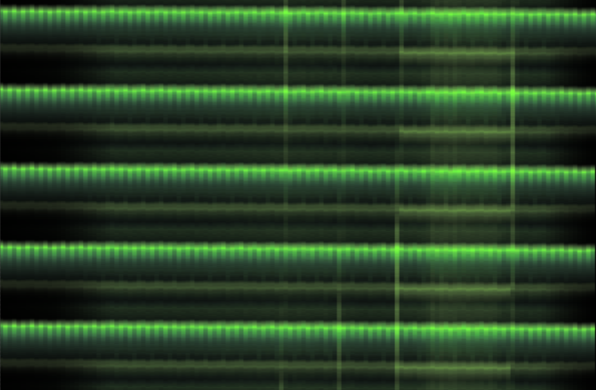
Lo/mid/hi bands
| ||||||||
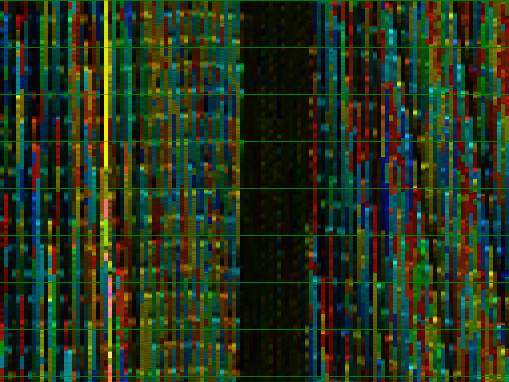
| Beatgraphs of a song (Not going home by Faithless, Eric Prydz remix) filtered throuhg a lopass, bandpass and highpass filter. |
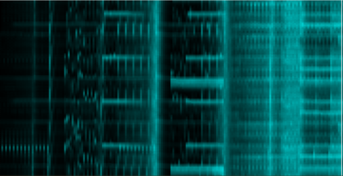
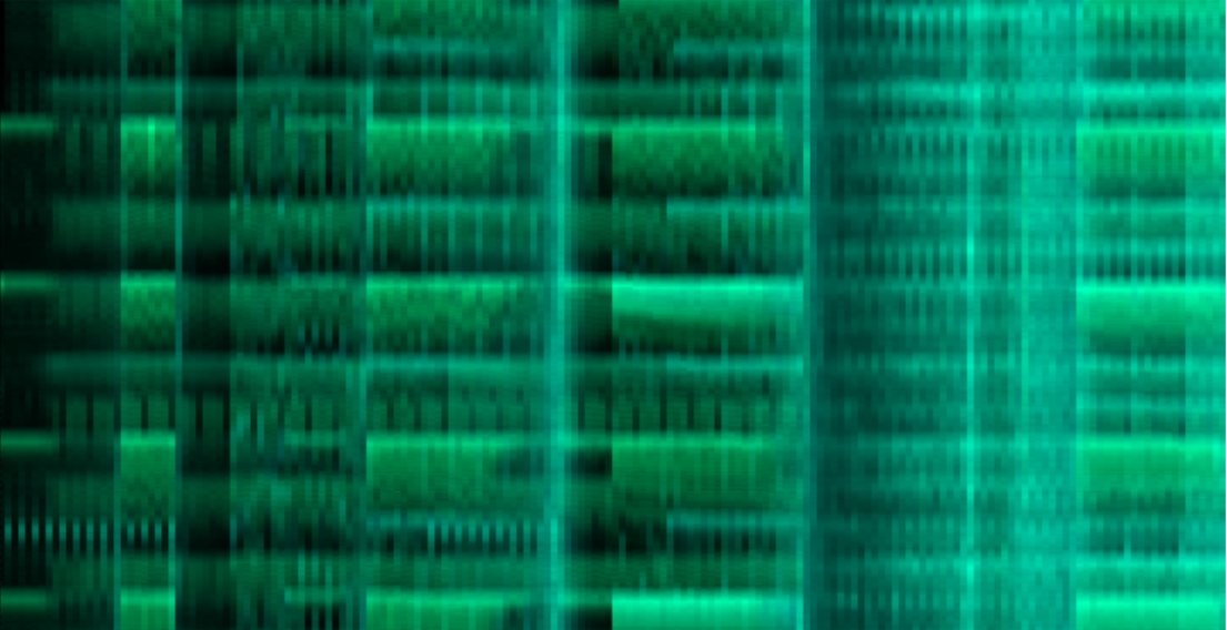
Because wavelets were too sensitive to the fine high-frequency time
resolution...
because they did not correctly represent the
perceived loudness...
and because mapping multiple frequencies
bands to a single color was non trivial,
we revised our approach
and created a set of 3 moving average filters with cutoffs at
the 8th and 16th bark band (2012). This results in a set of 3
images, which can be superimposed much easier. Using slightly different
hues is then often sufficient to differentiate between lo and hi
frequencies.
Self organizing maps
| ||||
| Coloring bars based on the cell number in a self organizing map |
A strategy we experimented with (2007) was to use a self organizing map [7] to cluster all bars. In this case we had a number of neural units. Each unit tried to describe a collection of bars that suited it best. Each unit was later assigned a hue which was then used to color the beatgraph. All together this was an expensive calculation and did not produce results that could be sensibly interpreted. Sometimes a bar was yellow instead of green, although the two bars sounded pretty much the same, etc. An extra problem was that it was difficult in advance to decide how many units we would need in our neural network.
Primary frequency based
| ||||
| Beatgraphs using the primary frequencies as color |
In 2009, BpmDj colored beatgraphs based on the primary frequency band. This made it possible to detect areas in the music that sounded the same. The coloring was different from the wavelet beatgraphs in the sense that we no longer assigned a color to each frequency; instead we found the main frequency and afterward decided on the color for each pixel, based on that primary frequency.
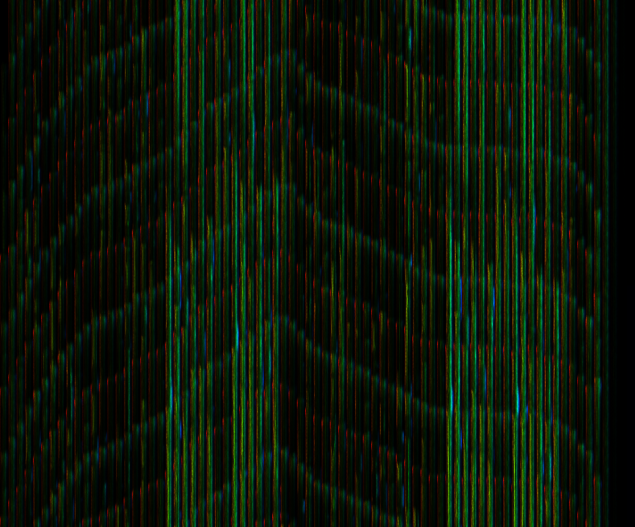
Multiband angular
 Beatgraphs in which the color is
deteremined using a ranking of the synthesized angles associated with
each frequency band (see text)
Beatgraphs in which the color is
deteremined using a ranking of the synthesized angles associated with
each frequency band (see text)
|
Because detecting the primary frequency bands was a bit too time consuming, we laid out a strategy that would combine the coloring advantage of knowing something about the frequency and the ease of using bandpass filters. In this strategy we used 6 bandpass filters, which were then combined to create a sense of what frequency range would be most dominant. Thereby we tried to reflect the primary frequency band. The frequency bands:
- Band 1 from 0 Hz to 400 Hz.
- Band 2 from 400 Hz to 920 Hz.
- Band 3 from 920 Hz to 1720 Hz.
- Band 4 from 1720 Hz to 3150 Hz.
- Band 5 from 3150 Hz to 6400 Hz.
- Band 6 from 6400 Hz to 15500 Hz.
Band splitting was performed using 4th order Butterworth filters. After extracting the 6 channels, a maxfilter [8] was used to determine the maximum energy within each pixel. This time we used a fixed beatgraph height of 192 pixels/bar. Once the 6 channels were present, they were individually scaled to fall within a 0:1 range. Once that was done each band was assigned an angle: e.g: band 1 is at 180 degrees, band 2 is at 150 degrees, band 3 is at 120 degrees and so on up to band 6, which is at 0 degrees. For each pixel we would then set out these 6 vectors, thereby using the energy as measured for their respective bands and sum them together. The result would be a new angle that was stored. This approach is somewhat inspired by a hodograph [9].
After this entire process finished we ranked them and assigned a value between 0 and 1. During the visualization stage, this number can then be mapped to any wanted hue value.
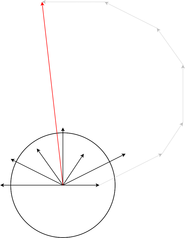 After assigning an angle to each band and retrieving the intensity of a pixel in that band (black vectors), we can sum all the vectors together (dotted gray). The result (red) provides us with an angle which is then interpreted as the frequency for that pixel.
|
When data contains a 2 dimensional array (band x time), then each hue value can be calculated as
for(int i = 0 ; i < L; i++)
{
  double hueX=0;
  double hueY=0;
  double max=Float.NEGATIVE_INFINITY;
  for(int c = 0; c < channels; c++)
    {
      final double e = song.data[c][i];
      final double a = (c * Math.PI / 5f);
      final double dx = (Math.cos(a) * e);
      final double dy = (Math.sin(a) * e);
      hueX+=dx;
      hueY+=dy;
      if (e>max) max=e;
    }
  hues[i] = (float) Math.atan2(hueY,hueX);
  intensities[i] = max;
}
Once done, both the hue and intensity arrays must be ranked
Considerations
Aspect ratios
 Same beatgraph at different aspect
ratios
Same beatgraph at different aspect
ratios
|
Because each beatgraph has a different number of bars to show, a valid question is whether we should generate images of a different size or force the width of the image to be the same in all cases. The former would produce pixels of the same size across different beatgraphs. This is valuable since we can then easily overlay beatgraphs. The latter method is valuable if we want to show a collection of songs. In that case the images should be of the same width, otherwise laying them out would result in a chaotic view. An extreme use of this is to replace standard wave-form displays. In that case the beatgraph will be shown quite broadly and with a very small height.
Intensity normalization
| ||||
| Griechischer Wein - Udo Jürgens |
The normalization of the brightness of the image can be somewhat challenging. Picking out the maximum intensity is often insufficient, because one loud click will make all other valuable content of the song go dark.
Another approach we considered was to pick out the maximum energy per bar and normalize each individual bar. At first sight that works, however a closer inspection reveals that valuable information becomes lost (in the above normalized picture it is difficult to find the refrain or see promptly where it is located). Also, areas where a break is, often come out in a chaotic manner.
Lastly, the approach that satisfies me most is to calculate the maximum energy in each window of 2 seconds and from all those values pick out the 97 percentile and use that as the maximum value. This approach has the benefit that
- it samples the entire song
- is not biased by how much empty space there is between beats
- cannot be easily thrown off by outliers
Hue / gamma correction
Given that the hues are not linearly spaced across the standard Java or Qt hue scale. Eg. Red, orange, yellow are three qualitatively distinct colors, but they are closer to each other than some other qualitative neighboring colors. Of course as explained in [10], how wide the secondary colors appear depends on the gamma correction. Thus, depending on LCD vs CRT, one might find that the beatgraphs appear qualitatively different. Although there is no magic bullet to solve this problem automatically, allowing the user to choose a certain gamma correction should provide the user with a handle on the problem.
Tuning the brightness to preserve transients
| ||||
| An example showing the difference between a plain and transient-normalized brightness |
A problem when visualizing modern songs is that certain types of music have the energy spread out everywhere. They are maximally loud and a beatgraph then tends to be fairly dense. Such music does however have transients. By correctly tuning the brightness one can bring out the transients while still preserving the overall loudness of the track.

The above equation explains how to convert a relative energy (between 0 and 1) to a pixel intensity, thereby retaining the overall loudness feeling (which is the 'e' term) and bringing out the transients (the 'e*e' term).
A more general form is one in which a variable alpha specifies how much transient we want to see
Saturation
A last aspect is that it is possible to add different levels of saturation to such image. One approach is to normalize each individual bar and use the saturation to reflect how much maximum energy is present in that bar. (This was done for the multiband angular picture above).
A better approach is to use the saturation to increase the brightness of the pixels, whilst still retaining the colored aspect of the beatgraph. This is based on the realisation that the color red, fully saturated has value (255,0,0), while the color red maximally 'non-saturate' is white (255,255,255). The non saturated colors are thus brighter than the saturated ones. Therefore it makes sense to map the energy of a pixel also to its saturation, but in the opposite manner: when a pixel has a lot of energy we decrease the saturation, when the pixel has less energy we increase the saturation.
| ||||||
| A sequence of beatgraphs. The enrgy range [0:maximumenergy] maps to the saturation values [maximumSaturation:0] |
When things go wrong
Of course, a correct beatgraph visualization depends on a correct analysis of 1) the bar length and 2) the start of the first beat. Tempo detection can be done as described in [11, 12, 13, 14, 15]. Rhythm detection can be done using a hierarchical decomposition of the extracted rhythm patten. This paper however does not address the analysis stage, merely how, once such information is known, beatgraphs can be visualized.
Notwithstanding it is useful to understand what happens if something went wrong during analysis
First beat wrong
| ||||
| Two beatrgraphs of the same song, but with different positions for the bar start |
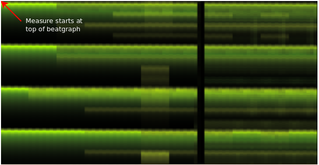
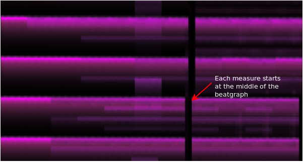
To plot a beatgraph fully correct one must know the location of the first beat in a bar. If that position is unknown then the beatgraph can still be plotted but might be offset somewhat. This results in a bar partly being drawn at the end of one visualized bar and then continued in the next. The above image shows this phenomenon. First beat detection can be done by means of spike detection in the difference between the future and past energy.
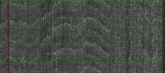
Tempo slightly wrong
| ||||
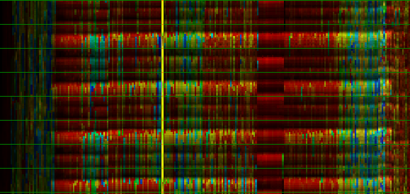
| The difference between a correct and incorrect measured tempo |
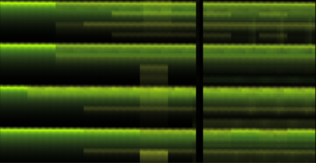
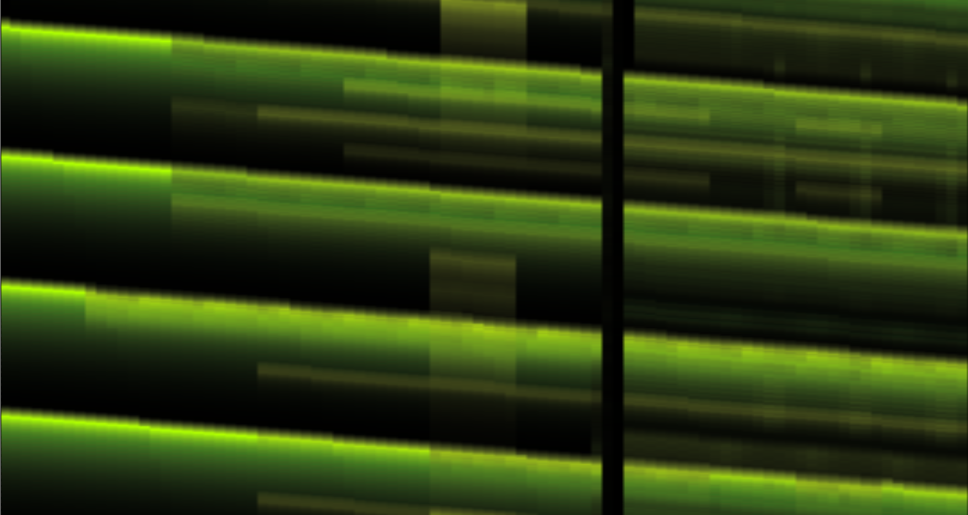
When the tempo measurement is inaccurate, each visualized bar will pull in a bit too much or too little information. And with each new bar the drift will become larger and larger. The result will be a slanted beatgraph.
Of course, in cases that the song does not follow a strict metronome, a beatgraph will look somewhat less straight. In those cases the beats will shift back and forth as time progressed.
Time signature wrong
| ||||||
| The same song (Dispensation - Andre Michelle), which is a 4/4 song, visualized as a beatgraph using various time signatures |
When drawing a beatgraph it is important to have the correct length of a bar. Since that length depends on the tempo (how many beats per minute) and the time signature (how many beats per bar), it is useful to know what happens if the time signature was estimated incorrectly
Conclusion
We presented a technique to visualize music, called 'Beatgraphs'. Although the essential idea is to visualize bars horizontally and the energy content of each bar vertically, there is a fair amount of leeway in choosing how to visualize the energy within each bar. When working in a monochromatic environment, the RMS visualization approach is probably the best. When working in a color-rich environment it all depends somewhat on how much space is available. Smaller spaces require a collapsed interpretation of multiple frequency bands, this can be achieved by using a complex ranking method based on a hodograph. When the images can be large, then each frequency band can be visualized as part of a dithering process. That leads to nice matrix-style paintings.
References
| 1. | DJ-ing under Linux with BpmDj Werner Van Belle Published by Linux+ Magazine, Nr 10/2006(25), October 2006 http://werner.yellowcouch.org/Papers/bpm06/ |
| 2. | BpmDj: Free DJ Tools for Linux Werner Van Belle 1999-2010 http://bpmdj.yellowcouch.org/ |
| 3. | Advanced Signal Processing Techniques in BpmDj Werner Van Belle In 'Side Program of the Northern Norwegian Insomia Festival'. Tvibit August 2005. http://werner.yellowcouch.org/Papers/insomnia05/index.html |
| 4. | Rhythmical Pattern Extraction Werner Van Belle Signal Processing; YellowCouch; August 2010 http://werner.yellowcouch.org/Papers/rhythmex/ |
| 5. | A Friendly Guide to Wavelets Gerald Kaiser Birkhäuser, 6th edition edition, 1996 |
| 6. | The Bark and ERB bilinear transforms Julius O. Smith, Jonathan S. Abel IEEE Transactions on Speech and Audio Processing, December 1999 https://ccrma.stanford.edu/~jos/bbt/ |
| 7. | Kohonen's Self Organizing Feature Maps unknown http://www.ai-junkie.com/ann/som/som1.html |
| 8. | Streaming Maximum-Minimum Filter Using No More than Three Comparisons per Element. Daniel Lemire Nordic Journal of Computing, 13 (4), pages 328-339, 2006 http://arxiv.org/abs/cs.DS/0610046 |
| 9. | The hodograph or a new method of expressing in symbolic language the Newtonian law of attraction William R. Hamilton Proc. Roy Irish Acad 3, 344-353, 1846 |
| 10. | How to Improve the Presence of Secondary Colors in Huebars used for Heat Diagrams ? Werner Van Belle YellowCouch; 5 pages; February 2009 http://werner.yellowcouch.org/Papers/huebars/ |
| 11. | Estimation of tempo, micro time and time signature from percussive music Christian Uhle, Jürgen Herre Proceedings of the 6th International Conference on Digital Audio Effects (DAFX-03), London, UK, September 2003 |
| 12. | Tempo and beat analysis of acoustic musical signals Scheirer, Eric D Journal of the Acoustical Society of America, 103-1:588, January 1998 |
| 13. | BPM Measurement of Digital Audio by Means of Beat Graphs & Ray Shooting Werner Van Belle December 2000 http://werner.yellowcouch.org/Papers/bpm04/ |
| 14. | Biasremoval from BPM Counters and an argument for the use of Measures per Minute instead of Beats per Minute Van Belle Werner Signal Processing; YellowCouch; July 2010 http://werner.yellowcouch.org/Papers/bpm10/ |
| 15. | Fast Tempo Measurement: a 6000x sped-up autodifferencer Werner Van Belle Signal Processing; YellowCouch; July 2011 http://werner.yellowcouch.org/Papers/fastbpm/ |
| http://werner.yellowcouch.org/ werner@yellowcouch.org |  |