| Home | Papers | Reports | Projects | Code Fragments | Dissertations | Presentations | Posters | Proposals | Lectures given | Course notes |
|
|
Biasremoval from BPM Counters and an argument for the use of Measures per Minute instead of Beats per MinuteWerner Van Belle1 - werner@yellowcouch.org, werner.van.belle@gmail.com Abstract : The peaks/valleys in autodifference/autocorrelation plots correspond to the potentially perceived tempo of music. Consequently, they can be used to measure the tempo of music. The problem with these techniques is the bias introduced through coherent noise. This bias is unique for each song and without its removal reported tempos might be off by a multiplication factor. This article discusses removal of such biases as to flatten out the autodifference/autocorrelation plots. Secondly, we discuss how the problem of tempo-harmonics (120 BPM reported as 90 BPM for instance) can be reduced from a multi-class classification problem to a binary classification problem. We also argue that the use of 'beats per minutes' is an artificial measure and should be superseded with the use of 'measures per minute', as it turns out to be a much more robust measure.
Keywords:
BPM measurement, BPM counter, bias removal, autocorrelation, autodifference, measures per minute (MPM) |
Table Of Contents
Introduction
In 2001 I created an algorithm to measure the tempo of digital music. The counter itself is quite accurate and the paper, although it was never published in 'recognized journals' due to gratuitous feedback from IEEE, has been accessed over 70'000 times by unique visitors since 2004 [1]. In this paper I would like to extend that work somewhat and look into a very specific problem with the counter: the counter is accurate, but it might report a multiple of the actual tempo (which we will call a 'tempo'-harmonic). For instance a tempo of 120 BPM can also be reported as a 60 BPM song, or even a 30 BPM song. This problem is common, but fairly annoying. In BpmDj this was solved -to a certain extent- by using only a tempo range from 90 to 160 BPM. Sadly, the multiplication factors are not necessarily whole numbers. They could as well be un(w)holy numbers. In practice we often found misreports that were 0.5, 0.75, 1.25, 1.5 or 2 of the actual tempo.
I have been aware of this problem and during the past 10 years I tried many an attempt to improve on this problem. None of these 'fixes' were really satisfactory. With a recent challenge, I became interested in structuring the old information somewhat as to get a better grasp on the problem and afterwards see whether we could break through and solve the problem of tempo-harmonics.
I first explain the various tempo algorithms that are currently in use in BpmDj [2, 3]. Afterwards, I'll focus on the new insights recently gained.
Current Tempo Modules
Autodifference / Rayshooting
'Rayshooting' is the essence of the previous paper [1]. I believe the best manner to explain the technique is by first assuming that we know the tempo and what type of visualization we can create based on proper tempo information. Afterwards, we turn this upside down and try to find the most satisfactory visualization, and (almost as a side effect), obtain the tempo by doing so.
Step 1: If we know the tempo of a particular song then we can extract all individual measure from the music. Each such measure can be visualized by drawing its energy content (high energy = white, no energy = dark) in a pixel-column. All these columns can then be placed next to each other, effectively leading to a 2 dimensional visualization of the music. From top to bottom one finds the content of each measure and from left to right the measures in consecutive order.
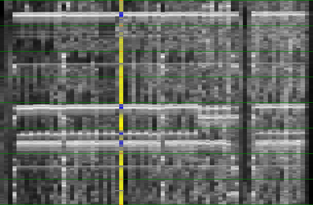
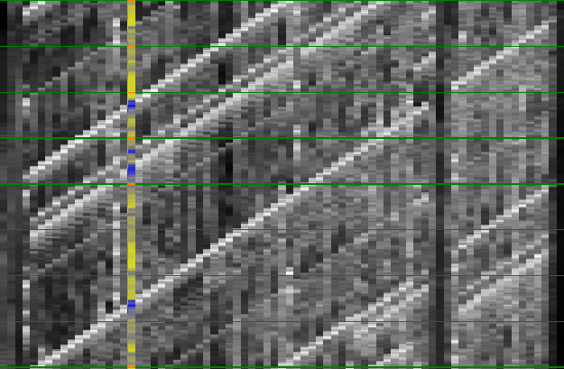
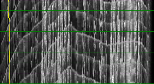
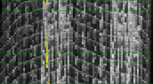
Now, if the tempo is measured correctly, the beatgraph should contain horizontal lines because each bass drum will be positioned at the same position on the y-axis. If the tempo is incorrect, then the beatgraph will be slanted as shown below.
| ||||
| The above picture shows how a song looks like if the time of a measure is properly known and when it is not quite correctly known. |
This type of visualization offers quite some advantages to Dj's. They can now inspect the song and see which areas offer the longest section of interrupted music, or they can in advance see when a break will arrive and mix in function of that [2, 3]. That is however not the focus of this paper. Here we want to know how to obtain the tempo.
Step 2: Obtaining the tempo is done by trying out all possible tempos and drawing the beatgraph. When the beatgraph is horizontal, we found the tempo. To measure the 'horizontallity' we shoot virtual 'rays' through the music. Each ray will 'shine' through the various measures and calculate how many mismatches it encountered. Horizontal beatgraphs will have a low average mismatch, while slanted beatgraphs will have a larger mismatch. Mathematically:

R_o,p is defined as the mismatch across all measures of the ray at offset o at a tempo of p. Hence, o is the position at the y-axis, while the 'i' in the formula scans from left to right and follows the x-axis. If we sum together the mismatch of the various rays then we have obtained the average 'horizontallity'. What is now looked for is the proper value of p (the period) that will produce the lowest r_p value. This constitutes a search problem as is demonstrated in the following figure. The figure shows how the proper tempo of a song is incrementally determined by scanning the song at various strides, while at the same time bracketing areas for the next search iteration. The details are given in the source of the standard 'Rayshoot' analysis module in BpmDj [3]
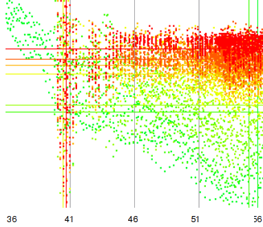 The different colors (from green to red) show the amount of
mismatch at a certain tempo and given a certain accuracy. The
green dots report on scans in a 1024 time down sampled song. The
slightly darker green dots report on the song down sampled by a
factor of 512. Each dot represents the mismatch. If it is high,
we have a lot of 'broken rays', if it is low we have a certain
continuity across the 2nd dimension. This figure illustrates
that finding the best ray constitutes indeed a search
problem. Initially it is not quite clear that the final tempo
will be around 41 BPM, and with each consecutive refinement we
find out that the best overlap is in a very narrow space.
|
I must admit that the wordchoice 'rayshooting' is maybe somewhat too metaphorical and nowadays I might prefer another more scientific term such as 'autodifference' to refer to this technique
Autocorrelation
A relatively known technique to measure tempo, is called autocorrelation. This technique appears to be similar to the presented autodifference (rayshooting), with the exception that we no longer calculate the absolute difference, but rather the multiplication of each two consecutive measures. This led some people to claim that our approach is merely autocorrelation (probably I was not part of their little gang). That is however wrong: the techniques are mathematically different. I will now elaborate somewhat further on such criticism:
1. A study on the properties of both approaches [4], shows that in general there is only a 0.6 correlation between this so perceived 'autocorrelation' (the sum of the absolute differences) and proper autocorrelation (the sum of the inproduct) in case of Gaussian distributed signals.
2. The main advantage of using autocorrelation is its expected speed. Given the proper Fourier transformations one can calculate the full autocorrelation in linear logarithmic time. A very satisfiable feature. The calculation of the autocorrelation is dependent of the execution of a forward Fourier transform, which will find the optimal combination of sine waves to produce the same signal. Of course, one believes that this first Fourier transform is somewhat sensitive to the energy in the song. That is however not correct, the presence of beats (which are waves at much higher frequency) does not constitute a good reason to perceive the very low oscillation (at BPM level). So, if we already measure something in the forward Fourier transform, then it is mainly a residual effect of the energy content around the various beats.
3. Autocorrelation, in practice, produces remarkable many tempo-harmonics. It actually only scores correct in 34% of the cases, while our own algorithm scores around 18% better. One could try to explain this as a result of the second inverse Fourier transform necessary to calculate the autocorrelation. In this step the phase information is removed and consequently, if we only had a couple of peaks, we will find new combinations of various peaks with each other. A form of synergistic effect between the various cleared phases.
[4. Calculating the autocorrelation of a song of 12 minutes requires a Fourier transform of 31 million samples. At this point we find that memory access as well as round off errors start come into play. How they affect the outcome is unclear, but the numbers one deals with are pushing the limits of the numerical sensitivity, although this is merely a technical remark]
Aside from the uselessness of direct autocorrelation, there are some worthwhile observations that could be used to our advantage later on. The following table compares the effects between autocorrelation and autodifference (rayshooting) when we compare two types of sound directly. Remember: the autocorrelation will/should report large values when the sounds are equal, while the rayshooter mismatch will/should report low values.
| First sound | Second sound | Autocorrelation | Autodifference (Rayshooting) | Comments |
| Beat | Nothing | 0 | Reflects the energy of the beat | both techniques are successful in penalizing this mismatch |
| Beat | Beat | Reflects the energy of the beat | 0 | both techniques are successful in obtaining a reward from the similarity |
| Noise | Noise | Centers around 0, but variance of the autocorrelation will be slightly greater | Reflects the combined energy of the two noise fingerprints | Both penalize the sound, which is wrong since noise has its place in music and is no longer an 'artifact' of the recording or so. |
| +2 DC | +1.5 DC | Although in the strict correlation sense this should report 0, autocorrelation will report 3, increasing the perceived similarity between these two sounds | 0.5, will decrease the perceived similarity between the two sounds | This is the single point where the two techniques differ qualitatively. In this case, the rayshooter performs properly because direct current is not something we perceive as sound. Aside from this, the rayshooter is also more robust. To illustrate this: assume the average in the sounds was not 2 and 1.5 but 10 and 9.5. The autocorrelator will report a much larger values in this case (95), while the rayshooter will still only report a mismatch of 0.5. |
| Nothing | Nothing | 0, lowers the perceived similarity | 0, increases the perceived similarity | This is a special case of the direct current example in the row above. Empty spaces in music appear between beats for instance. The rayshooter will weigh those similar empty spaces properly, while the autocorrelator will deal with them as if they are mismatches |
Fourier Analysis of the Envelope
Another widely known technique is a Fourier analysis of the envelope. This technique first converts the amplitude based signal to an energy based signal, using a sliding window that computes the RMS or average absolute value. Afterwards, the Fourier transform is let loose as to obtain the envelope spectrum.
If we have a song with a plain 4/4 rhythm then each beat will lead to a larger amplitude while the empty passages will lead to a lower amplitude. A Fourier transform can then figure out what type of sine we need to match the beats properly; thereby as a consequence reporting the tempo. The side effect of this technique is that one needs to have at least the 4 beats present, or we might need extra frequencies to get rid of the single unwanted beat, thereby leading to extra tempo-harmonics. Nonetheless, this technique in general produces much less tempo-harmonics, often (particular in techno) less than autodifference (rayshooting) in itself. The table below shows the results for a particular difficult dataset.
| Technique | % Correctly measured |
| Rayshoot | 53.06 |
| Autocorrelation | 34.69 |
| Envelope Spectrum | 48.98 |
| Envelope Spectrum * Envelope Autocorrelation | 47.96 |
| Rayshoot * Envelope Spectrum | 56.12 |
An interesting observation one must make here is that autodifference (rayshooting) and the energy envelope spectrum are somewhat opposing measures, with opposing accuracies. To understand this one must think about that what is actually measured. In the autodifference plot one measures the similarity between measures (4 beats in general), while the energy envelope spectrum aims to figure out the period between two beats. The energy envelope spectrum is not directly capable of comparing the various measures directly since there simply is no oscillation (sine wave) that spans full measures. Now, back to the accuracy of what we are measuring
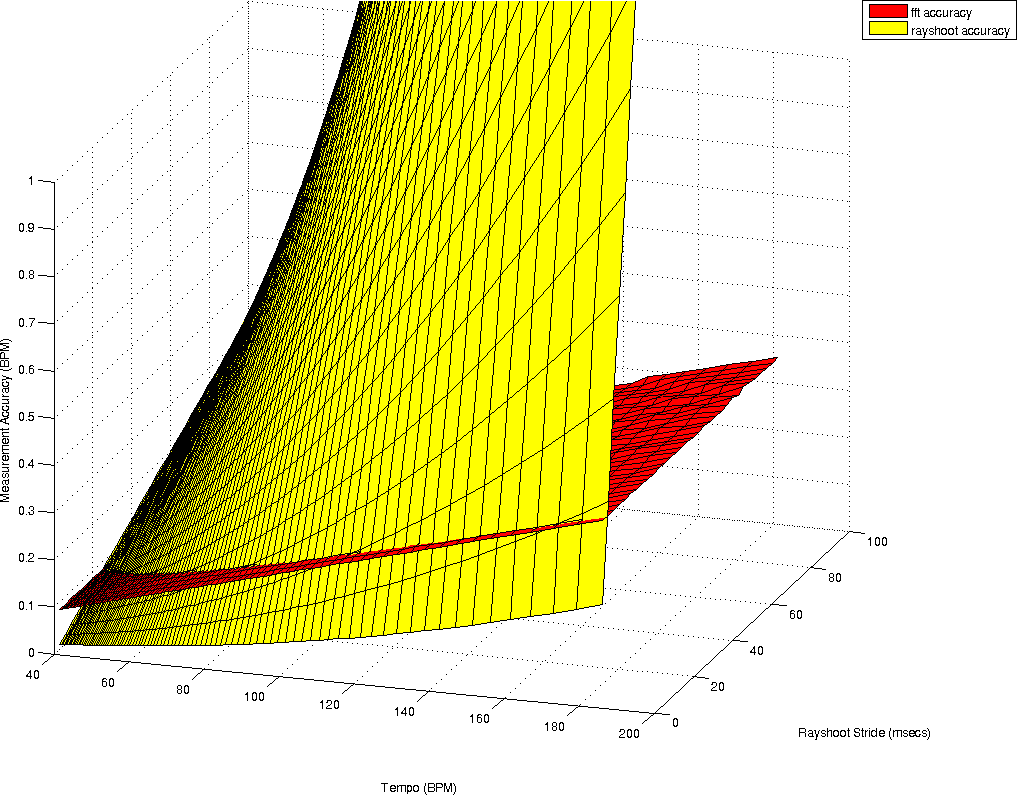
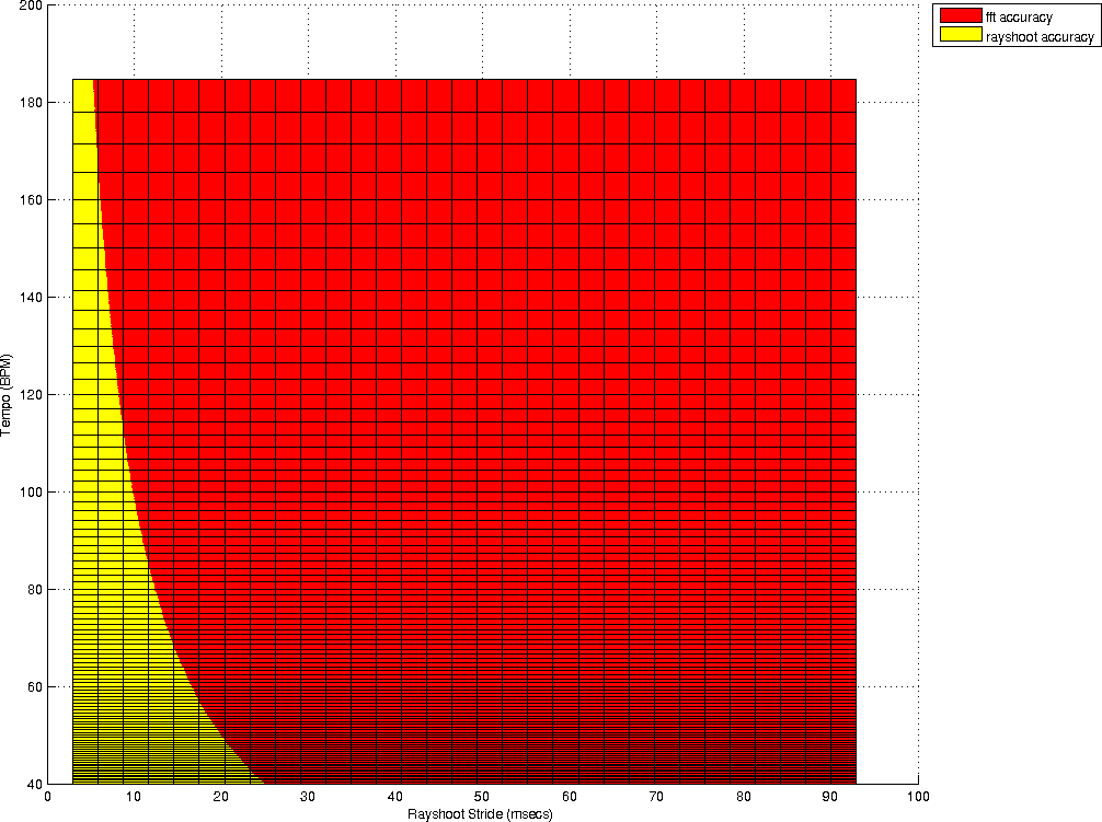
To document the accuracy of both techniques we calculate how accurate the tempo measurement is, given a certain windowsize. This is for the rayshooter the double of the period for one measure, which is itself already 4 times the period of a beat. So if we search from range 40BPM then we must have at least 12 seconds music (2 (we must at least be able to compare two measures) * 4 (beats per measure) * 60 seconds / 40BPM = 12 seconds). At higher tempos, the required fragment length is of course smaller. At a tempo of 180BPM, we only need 2.6 seconds. Once we know what tempo we can measure under a certain windowsize, the next measurable tempo depends on the stride used in the search algorithm. For the envelope spectrum only the windowsize is relevant and determines how accurately we can measure a specific frequency.
| ||||
| a) plots the accuracies of a tempo measurement at a given windowsize (for the Fourier transform) and a given windowsize and stride (for the rayshoot algorithm). Surprisingly, there is only a narrow range in which the rayshooter has a substantial higher accuracy. As soon as the stride increases, the accuracy drops dramatically. Figure b) illustrate the areas in which the rayshooter outperforms the Fourier analysis |
Of course, one should not be blinded by these numerical estimates of the accuracy, there is still one enormous benefit of the autodifference that is not offered in the envelope spectrum and that is that in order to compare two measures, we directly compare them, while in the envelope spectrum, such comparison is not present and mainly measures the presence of an underlying frequency. To make this clear: assume we have a particular shape of wave, which is not a pure sine wave, and which is repeated exactly from one measure to the next. The rayshooter will find no mismatch between the different measures, while the energy envelope will still find a variety of frequencies and might still have trouble finding this repetitive frequency.
Rayshoot mismatch & Envelope Spectrum
As a consequence from the above observation that a) the energy envelope spectrum often provides more useful information with regard to tempo-harmonics than the autodifference and b) that the autodifference provides more accurate tempo information, we tried to combine both techniques. This lead to a number of approaches. The first was a setup where the fourier transform would be used to guide the search algorithm.
The results of this approach were highly successful with a 56.12% success rate. There was however a problem in the implementation in that we could never find a sensible way to combine the two techniques. As soon as we multiplied the envelope spectrum with the rayshoot mismatch, we would loose the rayshoot accuracy. This is of course seems merely a matter of tresholding the fourier transform or directing the peaks better, but in this case, also the weighing of the various peak strengths would form a challenge. The figure below shows an example of such envelope spectrum guided rayshooter
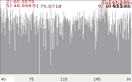 Guiding a rayshooter using the fourier transform of the envelope spectrum.
|
Envelope spectrum & Envelope Autocorrelation
Given the success of our previous combination, we also tried to combine the autocorrelation and envelope spectrum measures directly. This is done as follows:
- Calculate the envelope
- Calculate the envelope spectrum using a fourier transform after applying a hanning window over the song.
- Calculate the autocorrelation using the backward fourier transform
- Multiply the autocorrelation and the spectrum vectors
- For each potential tempo calculate the average of all multiple periods and report the tempo with the largest score
Reconsiderations
Before continuing, it is maybe time to rephrase some of the original issues involved. In particular, the entire notion of 'beats per minute' might be the wrong measure.
Humans are not even sure what the proper tempo is
Before delving into the algorithmic/mathematical side it is useful to point out the following, maybe obvious, but nonetheless important, observation:
There are a number of songs in which the rhythmical structure (beats, hi-hats) does not match the melodic structure. In particular, the song Bladerunner (by Vangelis) comes to mind. This has a very fast rhythmical structure while the melodic structure is very very slow. In such cases the outcome depends on the person judging the tempo: do they choose the faster or the lower possibility.
Some songs are almost impossible to assess: e.g: classical music has very complex rhythm changes, while other music, seems to be an oasis of pre/post-echoes, with very low attacks. One has no idea how to measure the overall tempo. The artists just seem to sing whenever they feel like it (Enya comes to mind).
Time signatures and "Beats" per minute
The time signature of a song specifies how many beats belong in 1 measure. Most songs have a 4/4 time signature. So, if we measure the length of one measure (something that is much easier than measuring the time between two beats), then we simply need to multiply it by 4. Now, of course, if we have a 3/4 time signature we should multiply by 3 and not 4. If we would still assume that the number of beats is 4, the reported 'beats' per minute will be wrong. So, once the measure length is obtained, one still has to figure out the time signature of the song.
This potential difference in time signature is one source of tempo-harmonics, since the previously reported BPM-counter [1] always assumes a 4/4 time signature. If it actually was a 3/4 time signature the tempo will be 33% off.
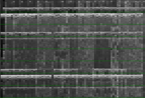 How many beats can you count ?
|
The use of such time signature is on the other hand an artificial construction; useful to create music; but not often does the music retain the 'beats' as such. E.g: how many true beats does each measure have in the picture shown left ? So, one should realize at this point that the beats per minute (BPM) measure refers to the construction of the music and to a lesser extent to the listening experience.
That of course poses the question: why are we then interested in 'beats per minute' ? Well, because tempo information is necessary to be able to mix music ! However, even if we have the BPM correct, given a certain time signature, it does not automatically make those two songs mixable. E.g: a 3/4 rhythm at 120 BPM and a 4/4 rhythm at 120 BPM tend not to be very mixable, although they have the same tempo. Stated differently: if the algorithm would report those two '120 BPM' tempos differently, it would actually not be making a mistake, since it would not make any sense to mix the anyway.
As a summary: 'Beats' per minute is an artificial measure, and there is no payoff to be expected on solving the time signature problem just to be able to report the wished for BPM. It would make more sense to get rid of this artificial construction and start counting the length of measures instead. Of course, counting the 'measures per minute' (MPM) will lead to unfamiliar numbers. E.g: a 120 BPM 4/4 songs, will be 30 MPM, while a 120 BPM 3/4 song will be 40 MPM. In order to keep some sense of familiarity it might be useful to always multiply the measures per minute with a factor 4 and then refer to the number of quarter measures per minute. (qMPM) One could also boldly redefine the BPM measure :-)
Investigating *1, *2, *4
With the various possibilities to obtain horizontal beatgraphs, one might wonder: which of the multiplicities of beatgraphs look good ? If we could find a mathematical definable property, we might be able to use that to guide the search. Let us have a look at a number of songs and see whether we can find such properties.
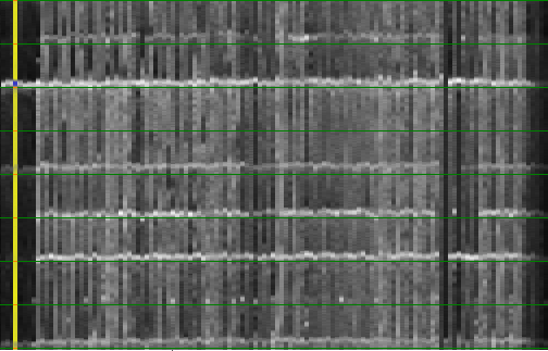
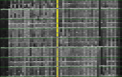
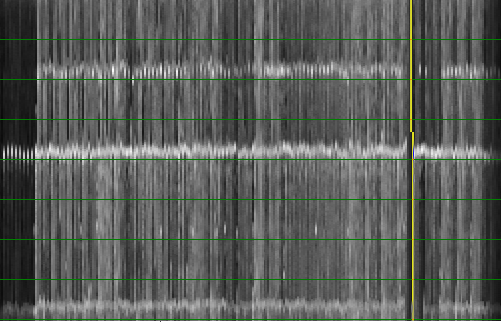
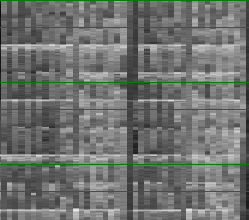
1st half measure = 2nd half measure => increase tempo ?
| ||||||
A song (Constant Craving - G.D.Lang) shown first at the tempo I would choose for the song (left). As we expect, we find nice horizontal lines and have a fairly straightforward overview of the content of each measure. We can obtain a similar graph if we halve the tempo, in this case we see two measures per vertical slice (middle picture). One could also perceive this to be the normal tempo. However, what stops us from concluding this is the fact that the upper half of the beatgraph is quite similar to the lower half of the beatgraph. Maybe as a rule we could state: 'if the first half of the measures is sufficiently similar to the second half of the measure, then the tempo should probably be increased with a factor 2.'
Of course, if one tries to express this mathematically, one finds that this exact measure is already incalculated. The calculation of the double tempo already compares the 'first' and 'second' parts of the measures automatically. So this rule is already present in the algorithm and it mainly seems to be a matter of weighing the mismatch-graph differently. (E.g: give more weight too smaller periods).
To finish this demonstration, we also show the beatgraph at a ridiculous tempo of 256 BPM (completely right). Here each 'measure' is actually only one beat. Although the tempo is way too high, it might be a sensible conclusion for an algorithm: lots of horizontal stuff going on here.
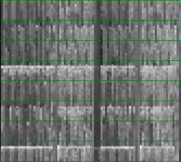
Interleaving => lower the tempo ?
| ||||||
A second idea was to look into the 'interleaving' of measures. The idea here is that certain songs at their natural tempo do not interleave, while, if we looks at them at a tempo that is too high, we find a lot of interleaving. Based on this we could try to create a rule that states: 'if we find interleaving, then we should lower the tempo.
So, what does this 'interleaving' means: it is essentially a graphical aspect of the beatgraphs in which we find that the odd and even vertical slices have their own makeup, and instead of finding a solid horizontal line for each beat we will find a dotted line. In the above pictures, the song Viva Forever (Spice Girls) is shown. Left, we show the song at a tempo which is too low, and we find again that the upper half=lower half. In the middle we find the song at its preferred tempo. Right we find the song at 168BPM, which is too high and we clearly see the interleaving under the form of dotted lines.
We might now be tempted to believe that we want to avoid such odd/even pattern in the beatgraph. This might be possible by first picking out the odd and then the even parts and checking whether we obtain a sufficient improvement on the overall ray-breaking. A form of permutation of the music before the autodifference. However, this is not necessary since this, has also already been incalculated in the rayshoot graph. We already know of the improvement on mismatch error in we would take the half tempo. So, despite an appealing approach, we already have the information in the mismatch graph. Beside, the idea itself not always works, as is demonstrated in the following example.
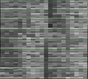
Interleaving might be wanted ?
Let us look into another example that shows a song where the interleave-avoidance strategy would not work
| ||||||
In this example (Walk Away - Aloha), we see that the tempo by which the beatgraph has the largest interleaving is also the natural tempo. In practice there are quite a lot of songs that behave like this. In other words: an 'interleaving' factor as measure doesn't seem to be very realistic.
Beats per measure should be around 4 ?
Another idea to consider, is counting the number of beats and assume that we want 'around 4 beats' in each measure. Below we provide three reasons why this will not work.
a) this proposed strategy will never be able to deal with the variety of existing time signatures (some time signatures only have 3 beats)
b)it is not clear how a beat is defined (a bass might look suspiciously similar to a beat, as pictured below. In this case the natural tempo (shown right) has around 8 beats per measure (it is actually a bass and not a bass-drum). The reason one chooses this particular tempo is that the melody is sung at a lower speed, which brings us to the crux of the problem with beatgraphs as they are: they do not really take the melodic content into account. Actually, they are remarkably insensitive to melody. A slight difference in frequency will not affect the rayshooter sufficiently to make a proper dent in the mismatch-plot.
| ||||
| Beatgraphs of the song 'Griegischer Wein (Udo Jürgens)' |
c) And finally, even if the song is a 4/4 song, beats are virtual entities used to create music and do not need to be present in the music.
Drift
Another important observation is that the tempo might not be strictly followed by the artist. Often the measures will drift somewhat around their average tempo. In that case one perceives a graph in which the 'horizontal lines' are far from horizontal, as already visible in the above pictures.
Intermediate conclusions
So far, we investigated both the techniques used to analyze music and a number of problem songs. Based on that we concluded the following:
- The time signature of a song determines the beats per minute (BPM), so it is crucial to be able to first measure the proper amount of measures per minute (MPM).
- The differences between interleaving and upper half=lower half considerations lies in weighing the various elements of the mismatch graph. We should investigate this weighing scheme in more detail.
- Melody matters and might bring a fast rhythm down to a more sedate experience. We should investigate the link between melody and perceived speed.
- Most music drifts and does not follow a metronome exactly. We should find a way to straighten out the music.
- We cannot expect an algorithm to perform 100% correct all the time; so whatever we come up with, it will involve some hand tuning to maximize the results as to satisfy our humane sense of 'tempo'. In this paper we will also mainly be looking into the problem of deciding on the correct measure length. The retrieval of time signature information is left as an exercise to the reader :-)
The mismatch-graph bias
As noted in previous sections: the decision whether we choose one peak (in case of fourier based approaches)/valley (in case of rayshoot mismatch graphs) over another depends on weighing the different tempos. We assumed -or one could assume- that the bias in the mismatchgraph is a systematic effect from the analysis and/or the measurement and merely linking a weight to a tempo might solve the problem.
First of all: it is true that there is a bias introduced through the analysis: if we assume a large measure, we will have few measures to compare, and consequently the mismatch will be lower. And in the opposite way: if we have a low period (= high tempo), the number of measures to compare increases, and thus the mismatch will increase. Luckily it is fairly simple to fix this problem. One simply counts the number of comparisons involved and divides the reported mismatch by that. This normalization can be compared to the biased and non biased auto-correlations. Sadly enough this is not sufficient to solve the problem (it would really have been too easy).
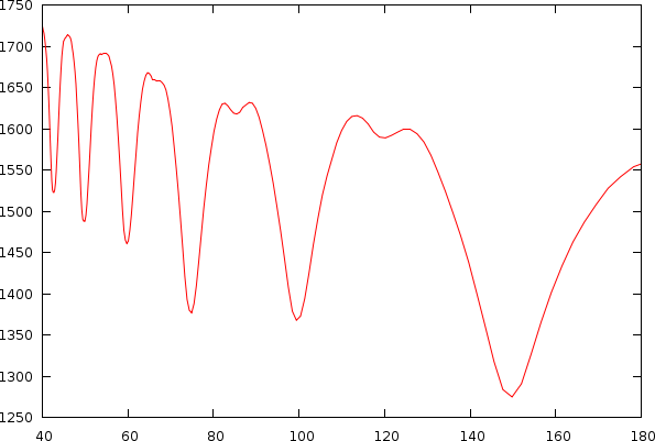
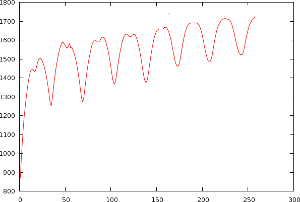
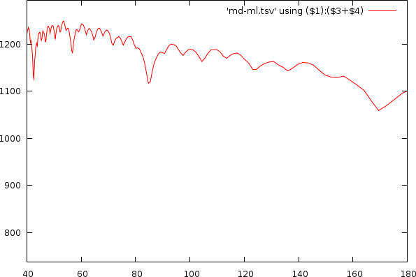
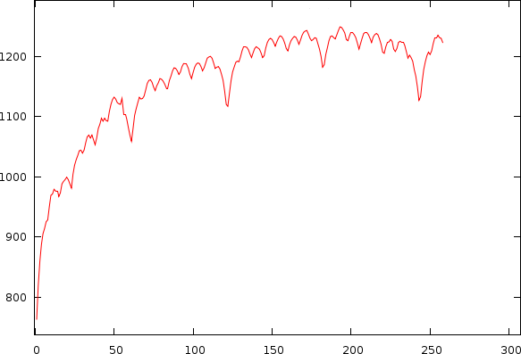
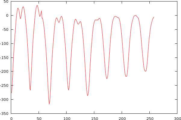
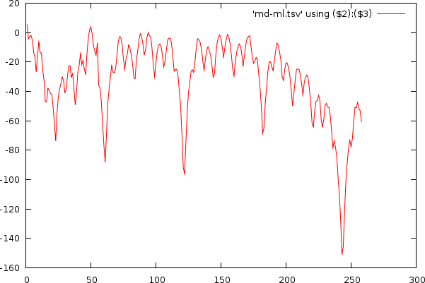
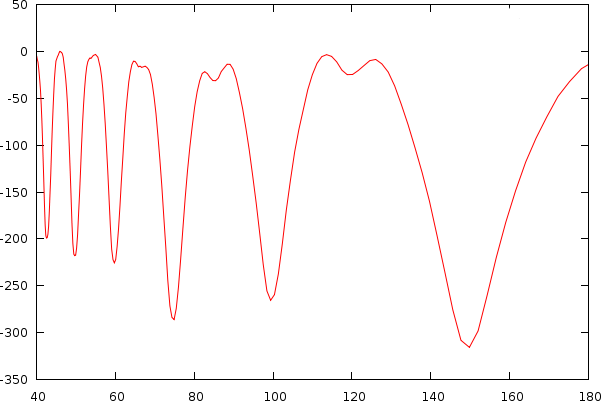
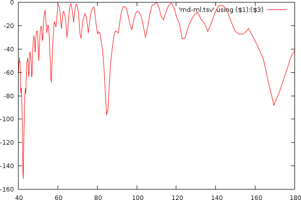
After observing many songs, we figured out that the bias is also unique for each individual song. This problem is directly apparent if we look into a couple of examples of mismatch-graphs whereby we also show periods starting from 0. As to illustrate its -less visible- effect on tempo, we also show the tempo and its associated mismatch.
| ||||||||
| The same song shown as a tempo to mismatch graph (left) and as a period to mismatch graph (right). One can clearly observe a number of potential hits in the mismatch graph. A and B: Griegischer Weinn - Udo Jurgens. C and D: Madonna |
To understand the biases slightly better, we can try to explain them by observing two types of songs.
The first type of song has a boring bass-drum ramming through the speakers for about 8 minutes. This type of music easily reports wrong multipliers. Humans of course assume it is a 4/4 key, however, there is no way for the algorithm to decide which peak it will be. (4 beats per measure, 5 beats per measure, 6 beats per measure appear all the same to the algorithm). The only thing that now guides the outcome is the bias itself. Consequently, the algorithm chooses the higher tempos.
The second type of music has a lot of structure and each measure and the whole composition is richly filled. One measure tends not to have the exact same information as the previous one. This provides for some interleaving in the beatgraph, which thus produces a higher mismatch than necessary for the correct tempo. In this case the algorithm will favor the lower tempos, and we have observed, that the depth of such valleys outweighs the bias often.
We tried a large list of potential solutions to normalize the mismatch-graph:- As a potential solution one could try to normalize the local 'valley' and its depth against the surroundings. The problem with this approach was that valleys at large periods tend to be broader, while those at large BPM's tend to be narrower but deeper. We could not figure out a sensible approach to solve this.
- It is known that the frequency content of the song automatically introduces a bias across all periods and it appeared possible to use the known spectrum of the song to normalize the bias introduced to similarities across the spectrum. We could not get this to work.
- After figuring out that the variance of the rayshooter is also dependent on the period under investigation we tried to use that to normalize the mismatch graph and relied on the lowest bound that would satisfy a 95% confidence interval. This lead to some success, however, the overall effect on the beatgraph was not as we wanted. Also, the certainty of a certain value does not necessarily relate to how we perceive the music and might be merely a mathematical curiosity.
- An observation we made during testing was that the bias was removed completely if we only measured y periods for every ray. independent from the period x itself. This indicated that the bias is merely a numerical issue in measuring the mismatch. A type of coherence noise. The more we measure it, the stronger the output of this type of artifact. Normalizing this can be expected to be difficult. As already pointed out, relying on a confidence interval to lower the mismatch for small periods didn't really satisfy us. We could also consider the other approach and increase the number of measurement artificially for lower periods. We did not test this because there simply is not enough data to fake the new measurements, and properly faking them by creating a probability distribution would account for a normalization method in itself. We decided that it might turn out faster to directly normalize the resulting graph instead.
- A possibility was to not report the average rayshoot mismatch per period (remember each period x has x rays to be shot through the song), but report the minimal mismatch, in which case we would essentially use this one ray as anker. Some good results but again very dependent on the mathematical structure of the music and not much related to our own perception necessarily.
- At this point we started to realize that the structure of the music itself is what affects the mismatch-graph its bias and in a sense is deeply connected to the music itself. So we started to experiment with a possibility to design an 'expected' mismatch-graph between tempos 40 to 180 based on all tempos larger than 180 BPM. This resulted in some success but introduced quite a lot of noise in the data. We might revisit this idea at a later stage. At the moment however it is not viable and did not improve the results sufficiently.
- Approximating the autocorrelation graph with an inverse exponential function and mapping this to the mismatch graph. This didn't work, and only recently I figured out that the normalization of spectra and that of mismatch-graphs have some important differences, which we describe later.
- Approximation of the mismatch graph by trying to approximate the tempo to mismatch function. This is closely related to fitting an inverse exponential to a dataset. It did however not work out properly due to 'outliers'. That is to say, the dips in the mismatch-graph throw of the exponential coefficient, leading to progressively worse errors.
- Approximation of the mismatch graph based on a logarithmic curve that would fit towards two parameters: a) the slope at period 0 in the mismatch graph and b) the average mismatch. This went a long way to a solution, but was still misguided through dips in the mismatch-graph.
- Creation of a normalization function based on the last maximal values
- And finally: approximation of the mismatch graph based on a log fit of the last maximal values in the period to mismatch function. This is currently the preferred solution since it delivers the best results so far.
Last retained maximum
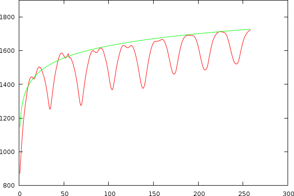
As already apparent in the two figures above, the mismatch-graph has a number of dips that are the focus of our attention. We want to keep these and not flatten them out. The mismatch-graph has however a bias (logarithmic in the period to mismatch graph and inverse exponential in the tempo to mismatch graph) which we want to remove because the absolute mismatch values might fall below other competing valleys through this bias (hence the tempo measurer might prefer larger tempos over smaller and so on. We don't like this type of bias). A strategy that works relatively well is to simply retain the last maximum value and thereby create a bias function, which will subsequently be subtracted.
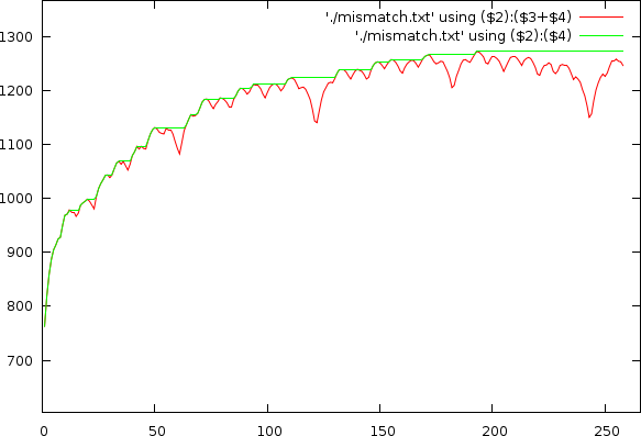 Mismatchgraph (red) and its propagated maximum value (green).
|
Logarithmic fit
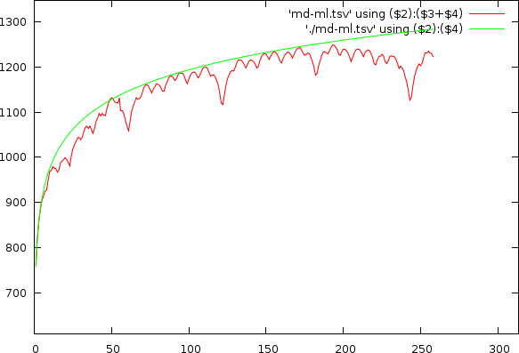
Because the biases under consideration appears as logarithmic functions, we aimed to create a logarithm that would go through a number of fixed values: We know that the mismatch at period 0 is 0 and that the mismatch at larger period must reach a certain value. So in a sense we aimed to create a logarithm in which we could tune the bend while keeping those two fixed values, well, fixed. The equation itself is parametrized by alpha (the bend) and beta, which is the scaling factor to ensure a maximal fit to the target.
Then based on the retained maximum graph, we calculate the mass of the non-normalized function and use that to make beta dependent on a through the indefinite integral

The results can be seen below
| ||||||||||||
| Udo Jurgens and Madonna, illustrating the estimated bias (green) on the original non-normalized mismatch-graph and the results in the tempo and period domain after normalization |
Melody Matters
Because it has become clear that the melody matters we might want to convert the audio sample first into a number of frequency bands, all of which are analyzed independently. Important on this filter bank is that it is very sensitive to the actual frequencies we are interested in. That means: frequencies between 50 and 3520 Hz, preferably spaced in accordance with notes.
To design such a filter bank we must of course take into account that we will use the output to calculate the tempo, meaning that the positional accuracy of the various notes should still be sufficiently high. For instance, the period of a 50Hz tone is 882 samples at 44100Hz, which means that to accurately measure the thing we need at least a window 2048 samples. However, if the rayshooter can only position a tempo accurately up to +/- 2048 samples, its accuracy will be reduced to 2.7BPM. Not something we should be overly happy about. On the other hand the speed of the search process will be drastically improved. As an intermediate solution, it is probably best to choose a stride of around 1024 bytes, independent of the employed windowsize. (It must of course be noted that our old algorithm [1] already used a boxcar average to scale down the music. However, it is also clear that such a simply lowpass filter is far from sufficient to properly deal with difficult scenarios).
The (somewhat naive) filter bank we currently work with is a sliding window Fourier transform that will stride over the music in blocks of 1024 bytes. The windowsize itself is independent from the stride, so we can at various different windowing lengths obtain sufficiently accurate measurements for a variety of notes. Currently we set up 6 different windowsizes that can cover the full notes A0 to A7. At window length 32768, we obtain note information for A0-F#0. At length 16384, notes G0 to F#1 are measured. At window length 8192, notes G1-F#2 are measured. At window length 4096, notes G2-F#3 are measured. At window length 2048, notes G3-F#4 are measured and finally at window length 1024, notes G#4 to A7 are measured. The last windowsize, which only needs 512 samples, was kept at 1024 sample, as to avoid loosing information. Secondly, 1024 bytes is only 23 milliseconds, which is sufficiently small to deal with in music.
Each frequency block (around 1024 bins) is afterwards converted to (on average) the 12 notes contained within that block. So we throw away a relative large amount of information and reduce the data size to about 8.3% of its original size. The frequency to note conversion works by calculating the note, selecting the proper bin and then taking the magnitude of the particular complex number. Once done, the collection of blocks, each covering a 48 notes, is further normalized through a logarithm, so that we can later on subtract notes in a psycho-acoustic sensible way. Once this is done all channels together are normalized. So in the end, we can without hesitation subtract information within one channel and the resulting data will be comparable to other channels; however, due to the normalization, we no longer know which basis was used for the logarithm.
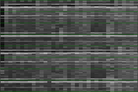
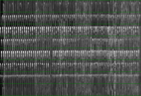
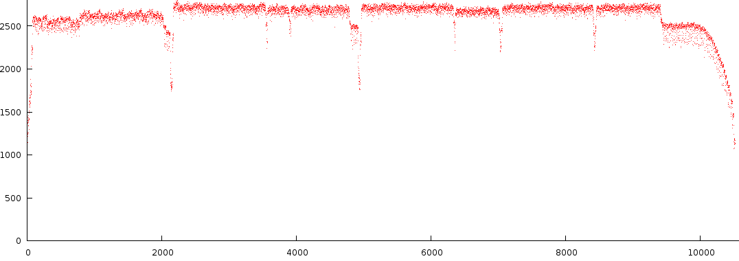
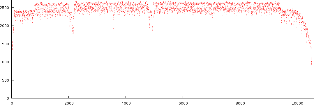
Below is the output of a number of notes from a specific song.
| ||||||||
There are a number of observations to this type of melody extraction.
- First of all the signal is not that dynamic. Most of the time its positioned near the top. Not something we necessarily want, however this is natural result from crosstalk between Fourier bins.
- The second observation is that in C3-B3, between block 6000 and 7000 we find two strengths back. A note at full strength and one at lower strength. This is interesting because it is something that is often overlooked in audio analysis.
- A third observation is that the dynamic range of a particular octave can differ from other octaves (compare C1-B1 against C2-B2).
- A fourth observation is that there seems to be a certain amount of noise present, something that, if we could, would like to get rid off, because, in layman's terms: 'either the guy sings or he doesn't.
- A fifth observation is that not a single note is truly off at any given time. This is also bad because it does not reflect how we perceive music.
Continuity in the melody lines
An algorithm we did some tests with was the possibility to smooth the melodic content of a channel so that it would have a lower variance and be more consistent.
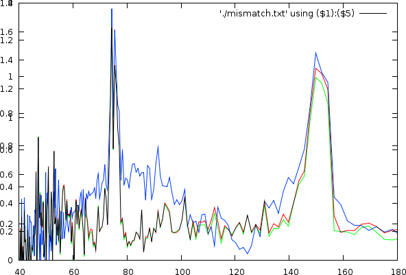 This figure shows the effect the smoothing of the melody lines
has on the tempo spectrum. Red is the normal spectrum, green is
if we use a window of 200ms and blue when we use a windows of
1000ms.
|
Edges in the melody lines
Together with the above, we introduced an edge detection that would calculate the absolute deviation and add it to the averaged signal, in this case, edges and change will become apparent as will the variance of the signal since the signal will be placed somewhat higher. This could potentially help discriminate the signal for the rayshooter. With respect to the frequency content we saw an even larger frequency bias in the tempo spectrum for large windows (but these we won't use since they will automatically prefer certain frequencies), and in case of the smaller windows (200ms), the effect was negligible.
The same held true for the rayshooter. For the smaller windowsizes, the mismatch graph improved slightly, with the biggest result coming from the smoothing. With large windows the effect was deteriorating the dynamic range of the mismatch graph.
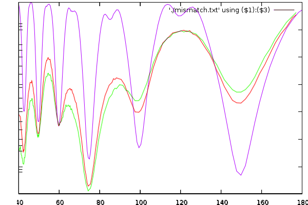 In this figure, the purple line is the normal signal (without smoothing). The green is using a window of 1s and the red one uses the same window but adds edge detection.
|
Possible other avenues
Although the melody extractor we currently use is not that satisfactory, it did improve the results substantially compared to [1]. The output mismatch graph was much smoother than we expected.
Notwithstanding, I strongly believe that the introduction of a proper melody extractor will improve the results even more. It is however quite difficult to obtain a proper one. Certain approaches start using neural networks to train a filterbank. And although this is cool we might even need to go further and develop a number of temporal bases (preconvolved comparators) to make this work properly.
Other options might be to normalize the melodic content across rays and not in advance. This could make a large difference in the measured outcome. Although in that case, we would merely take each rays, perform a principal component analysis. Select the 3/4 primary frequencies and then decide what the similarity is. This will require a lot of computational power.
Algorithms and Results
Given all the above information, we created a number of comnbiantion of autodifference and spectrum enveloppes (both normalized using our new technique) and thereby also relying on the melodyextractor.
An extra algorithm that was not explained yet is the use of a fouriere analysis of the period-graphs. As has already been aparanet, the autodifference and autocorrelation plots tends to repeat themselves somehwat. This repetition is always rtelated to a multiple of the tempo itself. The attempt here is to measure the rfequence of the autofdifference and/or autocorrelation plots. The problem with this technique is however directly the accuracy. ASuch 2nd order algotrirhm very quickly bumps into the limits of the song length and the blockszie of the extracted elements. Furthermoer, the results would remain questionable for songs that were otherwise questionable as well.
| Technique | % Correctly measured |
| Rayshoot | 53.06 |
| Autocorrelation | 34.69 |
| Envelope Spectrum | 48.98 |
| Envelope Spectrum * Envelope Autocorrelation | 47.96 |
| Rayshoot * Envelope Spectrum | 56.12 |
| Melody extracted autodifference | 30.6 |
| Melody extraction, Auto-difference (Maxlog fit) | 40.82 |
| Melody extraction, Auto-difference, attempted deconvolution | 32.65 |
| Melody extraction (Hanning), Auto-difference (Maxlog fit) | 45.92 |
| Melody extraction (Hanning), Auto-difference (Maxlog fit) * Envelope Spectrum | 62.24 |
| Melody extraction (Hanning), Auto-difference (Maxraise only) * Envelope Spectrum | 61.22 |
| Melody extraction (Hanning & edge detection), Auto-difference (Maxlog fit) | 27.55 |
| Melody extraction (Hanning & edge detection), Auto-difference (Maxlog fit) | 27.55 |
| Second order algorithm, direct Freq, measures choosen 4 times longer than need be | 45.65 |
| Second order algorithm. double pscan and maxraise normalisation for first and second order autodifference | 48.45 |
From the above tests we see that the logmax algorithm (as explained before) improves the results drastically. If we combine the output of the autodifference plot with that of the enveloppe spectrum, then our results become even more accurate. At this point we also started to realize that 100 songs was no longer a sufficently rich body of music to work with. A small change in the algorithms might bias the output of the algorithm towards faster or slower songs, potentially affecting 3 or 4 songs, and thus suddenly 'improving' the algorithm with 4%, while in reality our bias might have been created specially for the dataset we worked with. In other words: we needed to extend the musicbody and we needed to shift focus somewhat towards undertsnding the reported tempo-multiples better.
Setting up for classification in Slow / Fast music
Since we did not want to dwell too long on the problem of melody extraction, nor did we want to 'fiddle' with the algorithms to induce a proper bias for our particular musicbody, we started to think more along the lines of rhytm pattern extraction and learning to recognize specific time-signatures. That in itself posed a problem because one timesignature could often be measured through many tempo-multiples. To avoid that we needed a measure that would ensure a proper starting point to analyze rhythmical patterns
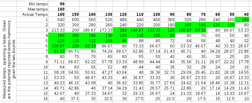
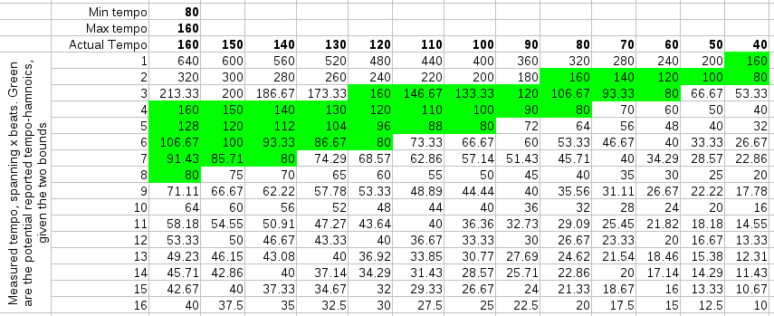
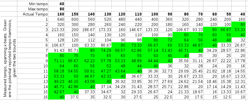
Below are three simulations of a straightforward 4/4 rhythm and what harmonics they might produce given our rayshoot algorithm: it measures the length of each 4 beats. To find the best tempo between 60BPM and 120 BPM, it will scan all mismatches between 2 and 4 seconds. This result is then converted back to a beats per minute range (divided by 4). Of course, while scanning these '4' beats, we will also find similarities at 3, 4, 5, 6,... beats.
| ||||||
| In the above figures, the actual tempo is given in bold in the columns. The rows contain the potential measurements. The cells colored green are those that fall within the scanrange (fall between mintempo and maxtempo). |
When scanning potential tempos, we reject those that fall outside the scanrange (or rather: the algorithm never looks at them), so the number of tempo-harmonics is limited by the tempo scanrange. Of course, the tempo scanrange also limits the answers one might receive. The actual tempo might not even be reported... So, what is needed is to obtain a proper tempo measurement and a multiplier that specifies how to map the measurement to the actual tempo. E.g: if the actual tempo is 140 BPM and we searched for the tempo between 40 and 100 BPM, the algorithm might report 93.33 BPM, in which case the reported multiplier should be 1.5.
From the above tables, we would expect more harmonics if we choose low temporanges and fewer harmonics with higher temporanges. That interpretation was however wrong when we tested it. The best scanrange was actually entirely the opposite of what we expected: 40-80 BPM or 45-90 BPM. This produces -to our surprise- either the *1 or *2 tempo-harmonic and very few other harmonics. Once one thinks about this it makes sense, because 'measures' are the more repetitive structure in music, while the internal measure structure tends not to repeat itself that much. By taking the longer windows, we also directly got rid of any interleaving effects we might otherwise be subject to. (As a sidenote: the fact that the observation in this case directly contradicted our expectation shows mainly that it is sometimes useful to test things instead of relying on silly spreadsheets.)
Actually the results of this unexpected temporange were so good
that we achieved 95% accuracy, when only allowing a *1 or *2
multiplier. Of course, if we do not allow an error in tempo-harmonic,
we only achieve 50% accuracy. It is however a serious improvement on
existing algorithms, since we no longer need to figure out whether we
must multiply the tempo with 0.25,0.66, 0.75 etc, we only need to
classify the music in 'slow' or 'fast'.
3/4th rhythms and 7/8th rhythms
The classificiation in slow/fast is one part of the puzzle of course, probably the most impoirtant partt. There is however still the problem that the BPM is a multiple of the MPM measure, which means that we still need the ability to find the number of beats that are contained within one such measure.
Conclusions
- We developed a normalization method to remove biases from mismatch-graphs. The mismatch graphs must be properly weighted before finding peaks. The bias present in each song can be modeled with a logarithmic function in case of the autodifference. In case of the energy envelope such fit is less optimal, but still necessary. Where the bias comes from is unclear and we are still not able to simulate it properly. Very likely the bias is the result of some form of coherent noise.
- We discussed some improvements on the rayshoot algorithm
- Melody influences the perceived speed of music. At the moment, we improved our rayshoot algorithm using a rudimentary melody extractor. This smoothed out the resulting graphs.
- The Autodifference and autocorrelation measure DC (direct current) differently.
- Combining the envelope spectrum and the rayshoot information is a useful technique.
- Noise is somewhat of a problem: it is a musical event that has meaning for humans but it confuses the crap out of the various algorithms
- We argued that 'beats per minute' (BPM) is an artificial measure used to synthesize music, which is not that suitable to measure tempo. Better is to measure the measures per minute (MPM) and then use the time signature to obtain the tempo. In some cases it might not even be necessary to go further than the measures per minute (E.g: mixing tools).
- We discovered a tempo scanrange that simplifies the problem substantially. With a scanrange of 45 to 90 BPM, we only obtained two potential tempo-harmonics: *1 or *2. This important result reduces the challenge to only a binary decision: is the song slow or fast ? (The original problem is a multi-class classification problem, where we can have up to 5 potential tempo-harmonics for certain measurements).
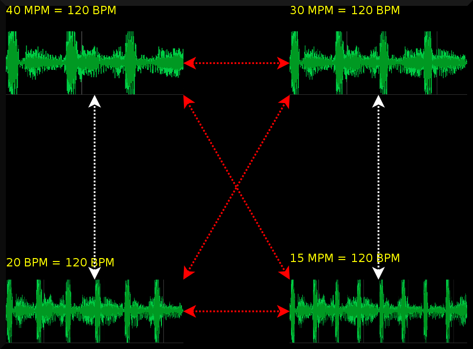
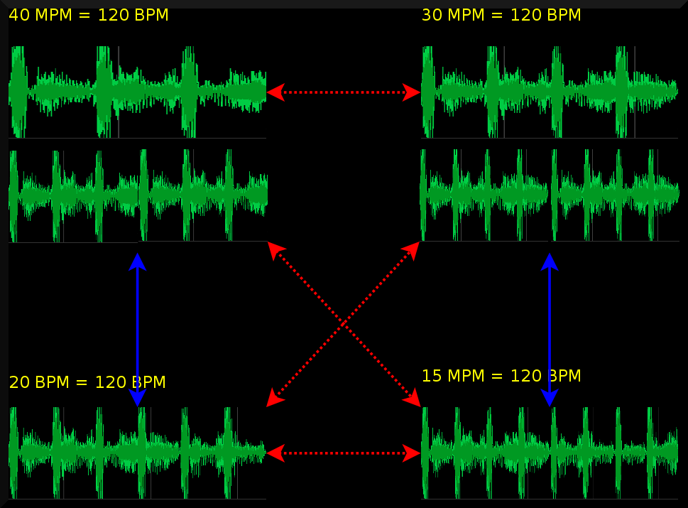
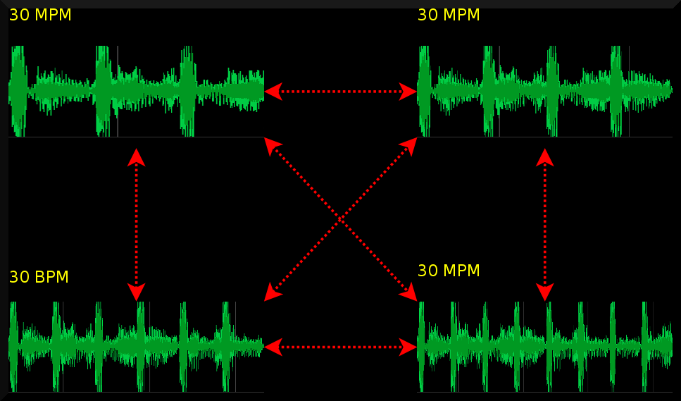 When the number of measures per minute are the same, but the rhythms different, then Dj software
can detect this incompatibility by comparing the rhythmical patterns
|
With the current incarnation of the algorithm, thereby allowing a /2 error, we achieved an accuracy of 95% on a test set of 300 songs. Future work will need to focus on solving this binary classification. However, in the meantime this result is sufficiently useful to start to use it in mixing software (this type of software is only interested in providing appropriate suggestions, not in understanding the philosophical finer points of whether something is truly a beat or not).
| ||||
| MPM different, but BPM might be the same. Such situations might occur when the tempo is in reality a double speed. In that case, shrinking the pattern and glueing them behind each other and then comparing towards a half tempo pattern resolves this type of problems. |
Future work
- Most humanly played songs drift. One might expect that such jitter or drift affects the outcome, and it does: it adds noise to the autocorrelation and mistmathc graphs; and we don't really have a good strategy to deal with them at the moment. Currently we simply ignore it and assume the maxlog normalizer will deal with it. And in practice this also works. So form thispoint of view it is a non-problem. However, if we want to continue with a heuristic that we can train to recognize certain timesignatures, and classify them into *1, or *2 tempo-harmonics, it becomes necessary that we clean up this jitter.
- The current melody extraction is very rudimentary. I believe that improvements in this areas will be beneficial to our algorithm
- Develop a neural network to recognize time signatures
- Develop a bayesian classified to do the same
- Try to us a radon transform to obtain even better tempo estimates.
Read further on how to extract rhythm information
Acknowledgments
I'd like to thank Günnther Rötter for providing me with around 200 testsongs.Bibliography
| 1. | BPM Measurement of Digital Audio by Means of Beat Graphs & Ray Shooting Werner Van Belle December 2000 http://werner.yellowcouch.org/Papers/bpm04/ |
| 2. | DJ-ing under Linux with BpmDj Werner Van Belle Published by Linux+ Magazine, Nr 10/2006(25), October 2006 http://werner.yellowcouch.org/Papers/bpm06/ |
| 3. | BpmDj: Free DJ Tools for Linux Werner Van Belle 1999-2010 http://bpmdj.yellowcouch.org/ |
| 4. | Correlation between the inproduct and the sum of absolute differences is -0.8485 for uniform sampled signals on [-1:1] Werner Van Belle Signal Processing; YellowCouch Scientific; November 2006 http://werner.yellowcouch.org/Papers/sadvssip/index.html |
| http://werner.yellowcouch.org/ werner@yellowcouch.org |  |
