11. Experiments

We have a habit in writing articles published in scientific journals
to make the work as finished as possible, to cover up all the tracks,
to not worry about the blind alleys or describe how you had the wrong
idea first, and so on. So there isn't any place to publish, in a dignified
manner, what you actually did in order to get to do the work.

- Richard Feynman, physicist, Nobel Lecture, 1966

IN THIS DISSERTATION, until now, we have explained how we can create a on-line working concurrency adaptor. This adaptor, however has not been created over one night. A number of different kinds of experiments has been performed. These experiments have highly influenced the current construction of the adaptor. Therefore, we feel it is necessary to explain these experiments in more detail. In this chapter we will give an overview of them. In the following chapter we will discuss the adaptor we have presented in this dissertation.

11.1 Introduction

Figure 11.1: Dependency graph of the performed experiments and developed tools. The orange boxes are development boxes. The green boxes represent the addition of extra information, such as Petri-nets, or component checkpoints. The blue boxes are off-line techniques. The yellow boxes are on-line techniques. Solid arrows are 'need'-dependencies. Dotted arrows are 'approach based on' dependencies.

PICTURE CONTAINS A dependency graph of the experiments performed and the tools developed. First, we designed and implemented the SEESCOA component architecture together with a controller that can startup a number of components and connect them to each other. This has been done in Java. Second, we created our own Petri-net evaluator and accompanying tools (pretty-printer, conversion to prolog, conversion to .dia^11.1 files, conversion to low level nets). Third, we implemented a large variety of test components (as specified in chapter 5), together with a Petri-net representation of their concurrency strategy^11.2. Fourth, we implemented a connection tracer that allowed us to verify whether the Petri-net was complete, hence that no message was not documented in the Petri-net. (described in section 3.6.3).

Below we will briefly summarize every experiment we have conducted. Initially we tried to create one adaptor to solve the concurrency strategy conflicts. However, after some experiments we took the decision to leave the track of off-line generated adaptors and focused on the practical usability of such an adaptor, hence we tried to make it work on-line. This posed some problems, which forced us to divide the adaptor in different modules as explained in chapter 7. The details of all experiments can be found on-line at http://progpc26.vub.ac.be/ cgi-bin/seescoacvs/component/concurrency/.

11.2 Experimental Setup

DURING THE EXPERIMENTS WE HAVE WORKED with two kinds of approaches. One approach was an off-line approach in which components are supposed to offer a test-component (pictured in figure 11.2). In such a setup, the learning algorithm has the opportunity to make wrong decisions which brings one of the participating components in an invalid and irreparable state. The second approach is an on-line approach in which a learning algorithm, or a learned algorithm, was supposed to work without failure. From both approaches, clearly the second is most realistic, because it can hardly be expected that in an open distributed system a component will offer 'test'-components, nor should any adaptor bring a component in an invalid state. However, as we have already explained in section 4.3.1, the off-line genetic approach offered some valuable insights into the representational problems we faced.

Figure 11.2: Setup of the offline strategy

11.3 Measuring Technique

AS EXPLAINED IN CHAPTER , every learning algorithm needs some kind of feedback. If we make use of an off-line strategy to generate an adaptor we should be able to measure how well that adaptor performs (the fitness) to solve the problem.

Measuring the correctness of a generated adaptor is not at all easy because it can be a Turing complete process, which means that we actually have to try it and cannot even see when it has stopped, or is executing in a loop and doing something useful. If we would have enough processing power available we could try testing all adaptors in parallel to each other. If we assume that all concurrent processes run equally rapidly we could measure every generated adaptor over a virtually infinite time span. All we would need to do is test all individuals concurrently and summing up the rewards as they are received. When a certain adaptor has become the worst it is killed and replaced by a new adaptor. However, this way of working has a major drawback: it is immensely resource consuming, both computationally and with respect to the memory requirements. [DK96,GW93] Therefore we will need to fall back to another approach.

To solve this problem of measuring a possible Turing complete process we introduce the notion of episodes. (such as in section 4.4.2). An episode is a finite run of a certain adaptor, that is an execution with a limited number of messages that should be handled. The amount of fitness received after this finite time is the reward for that episode. At the beginning of an episode the fitness is always zero (so the fitness of an adaptor does not take into account previous runs of the adaptor.). If at the arrival of a certain message the Petri-net of the adaptor goes into a loop, we terminate it after 2 seconds^11.3 and assign the current accumulated rewards as a fitness. If handling a message takes longer than 2 seconds, the component is killed. This technique of working is well known when working with learning algorithms, however often evaluation-steps are measured instead of real time. [Koz92]

The running time for every episode is increased slowly as the number of generations increases. By doing so we not only solve the resource problem of testing all algorithms at the same time, but we increase a number of interesting properties:

• With every new generation, every individual has to prove itself, thereby it can receive every time a better reward because the length of the episodes is increased. Therefore, any adaptor that has received once a good overall reward because it took a too specific action, will be removed very quickly in the following generations. For example: an adaptor that specifically works very well on position with $X-$coordinate 5, because the input expressions requires a 5 to be present at that place, will be removed in the following test round.
• Because the length of the episodes is slowly increased, the search-algorithm can find out solutions to new problems every time a new problem is offered. For example: the search-algorithm will first try to solve the problem of the Lock operation. A while later it will need to solve the problem of the Unlock operation.

Below we will chronologically explain every experiment we have performed.

11.4 Experiment 1: A Scheme Representation

Goal: Creation of one adaptor program between two conflicting concurrency strategies.

Means: Genetic Programming with Scheme as a programming language.

Deployment: off-line

Input: No Petri-net description of the conflicting concurrency strategies is present.

Output: Scheme program that is supposed to mediate two conflicting concurrency strategies.

11.4.1 Description

In this small experiment we tested how a Scheme program [SJ75] could be generated automatically that would solve the conflict of a nested locking strategy at one side and a non-nested locking strategy at the other side. Essentially, this is a very easy problem to solve for an adaptor. The only thing it has to do is keep track of a counter, which specifies how many times the client has already locked the resource at the server.

The operations of the genetic algorithm are scheme operations such as +, -, /, *, >, <, <=, >=, and, or, not, sendmessage, set!, define, if and handlemessage. The smallest solution we are looking for is given in algorithm 26. In the program, the first argument given to sendmessage is the port to which to send the message to.

11.4.2 Results

From this simple experiment we observed the following:

1. The random generation process was unable to create the above program. This is to be expected because the high number of basic operations, makes creating such a program very unlikely if done at random.
2. The random generation process highly influences the kind of generated programs. We could tune the process to generate this simple program, however, the algorithm would then be completely unable to generate anything else in other situations.
3. Measuring the fitness of an adaptor program is a discrete measurement, this means that the concept of 'gradually evolving to a correct working adaptor' is not at all easy.
4. The Scheme representation simply passes messages from one interface to another, it can barely handle the content of the messages, unless extra operators would be added, but if this were the case finding one suitable solution at all would become even more time consuming.
5. The lack of formal interface documentation was clearly observed in this program, because we had to supply the genetic algorithm with the terminals lock, unlock, lockResult and unlockResult.

11.5 Experiment 2: Classifier System Representation

Table 11.1: Parameters and characteristics of the genetic program

parameter

value individuals (genotype)

Goal: Create a concurrency adaptor between two conflicting concurrency strategies

Means: The Pittsburgh Approach to implement a genetic programming approach

Deployment: off-line

Input: Petri-net descriptions of two conflicting concurrency strategies & distributed fitness measure

Output: Classifier system to fill in the missing behavior

11.5.1 Description

Classifier systems (as described in section 4.3.2) are a well known technique to create algorithms by means of a genetic program. Because the Scheme representation suffered from too many problems, we changed our approach substantially. First we introduced a formal interface description under the form of Petri-nets, second we left the track of commonly used languages and investigated the use of classifier systems. In these experiments we were using the previous example of a non-nested versus a nested locking strategy. Both strategies offer simple enter/leave locking semantics. For a quick overview of the parameters of our genetic program we refer to table 11.1.

The goal of this experiment was to create a classifier system automatically (the Pittsburgh approach) that would mediate the differences between two conflicting concurrency strategies. The classifier system should reason about the actions to be performed based on the available input. Therefore we need to represent the external environment in some way and submit it to the classifier input interface. We have investigated the use of two different approaches to represent the external environment.

• Single message reactive systems: in a single message reactive system, the classifier system receives one message that declares the whole external environment. This includes the message that comes in, the messages that can be sent out and the state of the underlying component.
• Multi message reactive systems: in a multi message reactive system, the classifier system receives multiple messages. Every message specifies a piece of the environment. There are messages to describe incoming component messages, messages to describe outgoing component messages and messages that all together declare the whole state of the Petri-net.

11.5.1.1 Single message reactive systems

We now describe the semantics of a single message reactive classifier system.

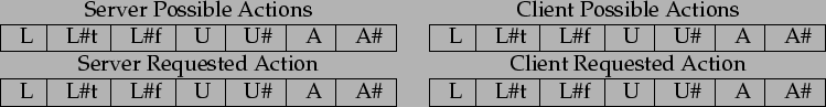
The input of a classifier consists of the full state of the client and the full state of the server, together with the actions which are required by either one of them. So, at first sight we should create messages which contain the state in which the Petri-net is in and the action requested by the client or the server. Of course, this would allow our classifier system to take invalid actions in a certain context. The classifier could for example decide to send an act message to the server when the server wasn't even locked. To avoid this we decided to represent the client/server state by means of the possible actions either one of them can perform. We can easily obtain these because we have a Petri-net model that describes the behavior of all connected components.

In the case of simple enter/leave locking semantics, we define the semantics of our messages as a 28 bit tuple (shown in figure 11.3), where the first 7 bits are the possible server actions, the next 7 bits represent the possible client actions, the next 7 bits represent the requested server action and the last 7 represent the requested client action.

Figure 11.3: L = lock; L#t = lock_true; L#f = lock_false; U = unlock; U# = unlock_done; A = act; A# = act_done. A bit is set when either a certain action is possible or a certain action is required.

With these semantics for the messages, simply translating a lock from client to server requires three rules (see figure 11.4). One which transforms the client lock request into a server-lock call (rule 1) and two which transform a server lock return into a client lock return. (rule 2 and 3).

Figure 11.4: The bit patterns from left to right and top to bottom: server possible actions, client possible actions, server requested actions, client requested actions. A description of the bit semantics can be found in 11.3.

Although this is a simple example, more difficult actions can be represented. Suppose we are in a situation where the client uses a nested-locking strategy and the server uses a non-nested locking strategy. In such a situation we don't want to send out the lock-request to the server if the lock count is larger than zero. Figure 11.5 shows how we can represent such a behavior.

Figure 11.5: Translating a client-lock to a server lock when necessary.

11.5.1.2 Multi message reactive systems

We now describe the semantics of a multi message reactive classifier system.

The message that resides in the input interface of such a classifier system contains a prefix that specifies what kind of message it is. When 000, the classifier message is about an incoming action from the client, 001 is an incoming action from the server, 011 is an outgoing action to the server and 010 is an outgoing action to the client. The prefix 10 describes the state of the client and 11 describes the state of the server.

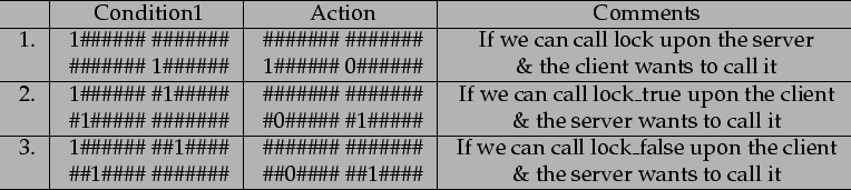
The rules of such a classifier system consist of a ternary string representation of the client state and server state (as specified by the Petri-net), as well as a ternary string representing the requested Petri-net transition from either the client process or the server process. With these semantics for the classifier rules, translating a request from the client to the server requires only one rule. Another rule is needed to translate requests from the server to the client (see table 11.2).

The number of bits needed to represent the states of each Petri-net depends on the number of states in the Petri-net as well as the variables that are stored in the Petri-net (e.g., the LockCount variable requires 2 bits if we want to store 4 levels of locking).

Table 11.2: Blind translation between client and server processes. The last 5 characters in column 1 represent the corresponding transition in the Petri net. The characters in the second and third column represent the states of the client and server Petri net, respectively. The fourth column specifies the action to be performed based on the information in the first four columns.

classifier condition

action

rule description requested

Although this is a simple example, more difficult actions can be represented. Consider the situation where the client uses a counting-semaphores locking strategy and the server uses a binary-semaphores locking strategy. In such a situation we don't want to send out the lock-request to the server if the lock count is larger than zero. Table 11.3 shows how we can represent such a behavior.

Table 11.3: Translating a client process lock request to a server process lock action when necessary.

classifier condition

action

rule description requested

In this experiment, which is an offline experiment, two components, with accompanying Petri-net descriptions of their behavior were offered to a genetic algorithm. The genetic algorithm would create complete classifier systems to link the two Petri-nets together. Initially, a single message reactive system was used, but as it turned out this classifier system was only able to learn very local behavior^11.4, therefore a multi-message reactive system has been tested. For the single reactive system, we will now define what our individuals are, how crossover and mutation happens and what we do to measure the fitness. These choices are standard choices for classifier systems.

Individuals are initially empty. Every time a certain situation arises and there is no matching gene we will add a new gene. This gene, which is a classifier rule has a matching condition with a random action on the server and/or the client from the list of possible actions. This guarantees that we don't start with completely useless rules which cover situations which will never exist and allows us to generate smaller genes which can be checked faster.

Mutating individuals is done by randomly adapting a number of genes. A gene is adapted by selecting a new random action.

To create a crossover of individuals we iterate over both classifier-lists and each time we decide whether we keep the rule or throw it away.

Fitness is measured by means of a number of test-sets (which has already been discussed in section 13.8.2). As explained, every test-set illustrates a typical behavior (scenario) the client will request from the server.

The genetic programming uses a steady-state genetic algorithm, with a ranking selection criterion: to compute a new generation of individuals, we keep (reproduce) 10% of the individuals with the best fitness. We discard 10% of the worst individuals (not fit enough) and add cross-overs from the 10% best group^11.5. It should be noted that the individuals that take part in cross-over are never mutated. The remaining 80% of individuals are mutated, which means that the genes of each individual are changed at random: for every rule, a new arbitrary action to be performed on the server or client is chosen. On top of this, in 50% of the classifier rules, one bit of the client and server state representations is generalized by replacing it with a #. This allows the genetic program to find solutions for problems that have not themselves presented yet.

The scenarios offered by the client are the ones that determine what kind of classifier system is generated. We have tried this with the test scenarios, as illustrated in figure 13.6. Scenario 1 is a sequence: [lock(), act(), unlock()]. In all scenarios, we issue the same list of messages three times to ensure that the resource is unlocked after the last unlock operation.

11.5.2 Results

Table 11.4: The generated classifier system for a single run.

requested

client

server

performed

transition

An examination of the results of several runs of our genetic programming algorithm lead to the following observations:

1. We found that (for all 100 runs of the genetic algorithm) a perfect solution was found within at most 11 generations. One of the classifier system that is generated by the genetic algorithm, when providing as input all test scenarios, is given in table 11.4. The produced classifier system simply translates calls from client to server and vice versa, unless it concerns a lock call that should not be made since the server is already locked. The bit patterns in the example differ slightly from the bit patterns explained earlier. This is because we need the ability to make a distinction between a 'transition-message' and a 'state-message'. All transition messages start with 00 and all state-messages start with 10 for client-states and 11 for server-states.
2. The best individuals were often created by only using mutation and creation of new genes. In the experiments we conducted we observed that the crossover operation is not necessary to find a suitable solution. This is because there are in essence not many parameters that work on the fitness independently. Another reason for this behavior is that the creation of new classifier-rules is based on a process that very actively selects a transition that is known to be enabled in a certain situation. Since most of the time not that many messages can be received or sent by a component, it is quickly checked in multiple generations which action is the best action in a certain situation.
3. About 50% of the created adaptors do not manage concurrency, but shortcut the missing behavior. That is, they offer the client a feedback behavior (such as the liveness module), without ever contacting the server.
4. The Classifier Representation of Petri-nets is Too Low Level: A problem with single message classifier systems is that their representation loses a lot of useful information. For instance if a rule has been found to lock one square in a clean way, it is not at all easy to extend this very specific rule to be a more general applicable rule. Unless the representation is very specifically suited to do that. This is especially a problem for the single message reactive classifier system, because the classifier system would need to invent an appropriate adaptor-strategy for every single square. This means that we have 1024 times more work than for one square. Above all it is not guaranteed that we will find a suitable strategy for all possible squares, because test-runs might not access all squares systematically. A solution to this problem would be to change a crossover operation and generalize one working set of rules to another set of rules, thereby taking into account the fact that repetitions occur at certain places. This information is available in the Petri-net, however, it is lost within the classifier system.
5. Classifier Systems have too Low Level Operators: In another experiment we tested the multi-message representation. After investigating this representation it became clear that it also was not suitable to do the job. This representation would allow the genetic program to find a suitable conversion strategy that could translate all incoming lock request to outgoing lock request in a way that would be automatically generalized. To allow this the coordinate of both the incoming and the outgoing lock-request was encoded within the bitstream at the same position. Nevertheless, if there would be a slight shift within the representation of incoming or outgoing lock requests (e.g: the incoming $x$ of a lock is located on bits 3 to 11 and the outgoing $x$ is located on bits 5 to 13), then it would become nearly impossible to find satisfactory classifiers. In general, the problem with classifier systems is in general that their basic operations are very basic, there is not even a notion of a variable.^11.6

In general these results lead us to conclude that classifier systems offer too low level operations and are unable to exploit structural properties of the presented interfaces. These problems are recognized by [SS89]. Therefore, we investigated another representation: adaptors with an internal Petri-net representation. By doing so we hope to take advantage of a) the structural knowledge present in colored petri-nets and b) make use of better high level operations.

11.6 Experiment 3: A Petri-Net Representation

Goal: Create a concurrency adaptor between two conflicting concurrency strategies

Means: Genetic Programming using Petri-nets as a representation

Deployment: off-line

Input: Petri-net description of two conflicting interface & a distributed fitness measure

Output: Petri-net that links the different interfaces

11.6.1 Description

In this experiment, which is again an off-line experiment, another representation was chosen. To avoid the problems of the classifier systems, we now create a high level Petri-net description that will be measured at runtime. The runtime measurement is still distributed and contains two parts. On the server part, it keeps track of how many errors occurs and warnings that happened. On the client side the fitness is measured at how many locks could be obtained. The representation itself is already detailed in section 9.1.

11.6.2 Results

Table 11.5: Experimental results of the priority-first searching algorithm, using the petri-net representation described in the text.

Component

# generations

Best Fitness

Transitions

Comments BallActor1

The results of this experiment were promising. First, we noticed that this representation had no problem at all to find out transitions to offer a correct 'mediated' behavior. Furthermore we noticed,

1. that random aspects within the components behavior quickly leads to correct solutions, while static behavior often leads to more narrow behavior.
2. Individuals resulting from crossover operations quickly die.
3. Most generated adaptors do not manage concurrency, but rather manage it to keep the involved components alive. It becomes clear that this is due to the non correlation of the two fitness measures (a fitness measure at client side and a fitness measure at server side).
4. If we modified the fitness measure, to include correlation of the different fitness values, we observed that other solutions were found. However, it was very difficult to create a suitable fitness function that guides the algorithm to an 'adaptor' solution. This problem has to do with the fact that measuring the working of an adaptor is very difficult and very conflict dependent.
5. Some adaptors implemented a feedback behavior that resulted in livelocks. From this experiment, we have observed that the liveness requirement is essential.
6. Comments with respect to figure 11.5:
   1. With this actor we introduced a delayed reward. Only when a SetPosition could be executed to move to the right or the left, a reward is assigned. This requires the search algorithm to test out a number of different tracks until finally a reward can be assigned.
   2. This adaptor works with two layers, hence the 4 transitions and different situations that can be encountered.

With respect to the before mentioned experiments two things became clear. First: we have found a suitable representation to express adaptors, however this representation does not easily produce concurrency solvers. Second, concurrency problems can barely be measured, therefore we started investigating how we can modularize the adaptor. To this end, we have split the behavior of the adaptor in three separate modules, as described in chapter 7.

11.7 Experiment 4: Bypassing a Provided Concurrency Strategy

Experiment: Automatic deduction of reachability analysis

Means: prolog conversion from Petri-net description and prolog analysis

Deployment: off-line

Input: Petri-net description in prolog and a required marking.

Output: A transition to execute to come closer to this marking.

Description: The description of this experiment is entirely contained in chapter 8.

Results: We have tested the working of this adaptor with relative markings and with absolute markings. To obtain absolute markings, we ran a number of test-components which produced an absolute marking from a real-life situation, afterward the prolog analyzer needed to find out how to enable that specific situation. In all cases the results were almost immediately known.

11.8 Experiment 5: Liveness and the Bucket Brigade

Experiment: Module to keep a client-component alive

Means: Classifier systems, the BBA and the earlier developed Petri-net Representation

Deployment: on-line

Input: Petri-net description of an interface, check-pointed component

Output: New transitions that will compete to keep the client component alive

Results:

1. The BBA is problematic because it specifies the mean future reward instead of a maximum future reward
2. One of the problems the BBA has, is that newly added transitions need an initial strength. If this strength is too low, the transition will be removed in the next step, without it having the ability to prove itself. If the strength is too high, slowly, good working transitions are flushed from the system. This can happen in situation that a new transition is never verified. To solve this problem we had to add a fairly difficult aging system, in which the strength of classifiers was determined based on their age.

After introducing the aging system to allow new rules to prove themselves, the similarities with reinforcement learning became clear.

11.9 Experiment 6: The Liveness Module and a Petri-net Representation

Experiment: Module to keep a client component alive

Means: Reinforcement learning, together with the earlier presented Petri-net representation

Deployment: on-line

Input: Petri-net of the interface, check-pointed component

Output: New transitions that will compete to keep the client component alive

Description: In the experiment, we use a number of different components, with different checkpoints, that will assign rewards as certain checkpoints are met (see section 9.2, page ). We will not document where these checkpoints are set due to space considerations.

Results:

1. Numerical results and a discussion of them have already been given in section 9.4.1.
2. Works very well in all cases, but one. Delayed rewards form no problem at all.
3. If the reward function has hidden correlations which highly influence the reward, thus the problem being not a Markov Decision Process, the learner has much more difficulties finding out what is exactly required.

The representation we use in this experiment, together with the reinforcement learning approach seems suitable for the problem we are dealing with. In all tests a satisfactory keep-alive program would develop quickly. In comparison to the classifier representation it is easy to swap two arguments or to increase the value of an argument. In our Petri-net representation this is easy because a) we have variables which add an extra level of structuring (the algorithm will find one solution for all squares on the whiteboard instead of one solution / square) and b) the operations at our disposal are of a sufficiently high level to be useful.

11.10 Implementation

The implementation of all these experiments, together with the results are available online. We didn't put them in appendices because this would require around 400 extra pages.

• *.component files need to be compiled to .java files by using the component system compiler.
• *.jjt files need to be compiled with jjtree
• *.jj files need to be compiled with javacc
• *.java files need to be compiled with javac (watch the CLASSPATH environment variable)
• *.l2net files are colored Petri-nets described in text. They should be converted to low level nets by the Petri-net compiler.
• *.l1net files can be used as input in the Petri-net evaluator
• *.ini files are input to the component system controller

11.10.1 The Component System

Runtime; Location: http://borg.rave.org/cgi-bin/seescoacvs/component/system/*

Runtime; Files: Component.component, ComponentSystem.component, AbstractPort.java, AbstractMultiport.java, AbstractPortCreator.java, ComponentImpl.java,  
ComponentImplFactory.java, Connection.java, DirectPort.java, ExecutionLoop.java, Global.java, InterruptHandler.java, InvocationMessageHandler.java, Message.java, MessageDispatcher.java, MessageHandler.java, MessageHandlerCreator.java,  
MessageQueue.java, MultiPort.java, Port.java, SameHandlerCreator.java,  
Scheduler.java, SetupPort.java, SinglePort.java, StandardScheduler.java,  
State.java, StreamAble.java, StupidScheduler.java, SymbolTable.java,  
ThreadedInterruptHandler.java

Compiler; Location: http://borg.rave.org/cgi-bin/seescoacvs/component/parser/*

Compiler; Files: Transformer.jjt, SimpleNode.java, and a large amount of parser node definitions. These start with Ast.*.

Controller; Location: http://borg.rave.org/cgi-bin/seescoacvs/testcases/scss/*

Controller; Files: Controller.component, ConnectionProxy.component,  
ContractGenerator.component, ReceivingMonitor.component,  
SendingMonitor.component

11.10.2 The Petri-net Evaluator Code

Location: http://borg.rave.org/cgi-bin/seescoacvs/component/concurrency/*

Evaluator: PetriNetEvaluator.java, PetriNode.java, StaticNet.java,  
DynamicNet.java, ExecMessage.java, ExecutionTrigger.java

Places: Place.java, SinkPlace.java, SourcePlace.java

Transitions: Transition.java, InTransition.java, ArcEntry.java, InputEntry.java,  
MessageTransition.java, OutTransition.java, OutputEntry.java

Expressions: AgAddOperator.java, AgAndOperator.java, AgCombinedExpression.java,  
AgEqOperator.java, AgExpression.java, AgField.java, AgForeach.java,  
AgGlueOperator.java, AgGrOperator.java, AgIdentifierDescription.java,  
AgIdxOperator.java, AgInteger.java, AgMessage.java, AgMulOperator.java,  
AgNotOperator.java, AgOperator.java, AgRange.java, AgSet.java,  
AgSubOperator.java, AgToken.java, AgVariable.java, Applicable.java,  
Bindings.java, EqualsExpression.java

Parser & Convertors: PetriNetParser.jj, Printer.java, PetriNet2Prolog.java,  
PetriNetConvertor.java, PetriNetSimplifier.java, PetriNetNormalizer.java

11.10.3 The Adaptor Code

Location: http://borg.rave.org/cgi-bin/seescoacvs/component/concurrency/*

Using classifiers: Adaptor.component, ClassifierCondition.java, ClassifierList.java, ClassifierMessage.java, ClassifierMessageList.java, ClassifierRule.java,  
ConcurrencyCase1.java, ConcurrencyCase2.java, Gene.java, MessageArgument.java,  
Scenario2_1.java, Scenario2_2.java

Component link: MessageDescription. java, MessagePlace.java,  
MyInvocationMessageHandler.java, MyInvocationHandler.java

The Pittsburgh approach: NeglectSynchro.component, PetriNetGenerator.java,  
PetriNetAdaptor.component, PetriNetLoader.component, PetriNetCrossover.java,  
PetriNetTimer.java, PetriNetCombiner.java, StandardLoader.component

The liveness module: FitnessAction.component, LearningAdaptor.component, 
ReinforcedAdaptor.component, GewogenPlace.java, GewogenTransition.java,  
PtReceiver.java

The enforce action module: anal.pl, ForceAction.component, ForceAction1.component, ForceAction2.component, PetriNetBackTracker.java

The concurrency module: SynchroAdaptor.component

11.10.4 The Actor Components

Location: http://borg.rave.org/cgi-bin/seescoacvs/component/concurrency/*

Shared Classes: ConcurrencyException.java, ActorRoot.component, Pos.java,  
ThreadCatcher.java

Server Components: PlayFieldView.java, PlayfieldCore.component, Square.java

Client Components: Actor*.component, BallActor*.component, FloodActor*.component, LineActor*.component, Actor*.l2net

11.11 Summary

IN THIS CHAPTER we have reported on the experiments we have performed. Our solution has changed over time from an initial scheme-representation of a concurrency adaptor, to a modularized reinforcement learning Petri-net adaptor. The path we have followed is a standard, 'prototype, experiment, observe, adjust' cycle in which mistakes are corrected in later experiments.

The experiments have allowed us to understand that creating a learning algorithm that will immediately create a concurrency adaptor is not possible, because the no-race requirement is very difficult to express and to validate.

We also learned that an off-line strategy offers certain advantages to verify the quality of the representation. We tried four different representations of an adaptor before a suitable one was found. These are, a scheme representation, a single message reactive classifier system, a multi message reactive classifier system and a Petri-net representation. Because the latter suited our needs, we stopped investigating which representation should be used.

However, afterward we turned our attention to the off-line/on-line problem. All the experiments initially conducted used an off-line strategy. However, from a pragmatic point of view, it is very unlikely that an off-line strategy can be made to work in an on-line environment. The main reason for this is that, once an off-line strategy becomes fixed in an on-line environment it might be unable to learn what to do in new situations, which have never been present in the off-line context. Therefore, we turned our attention to an on-line learning strategy, under the form of reinforcement learning. This turned out to be a very satisfactory approach.

Footnotes

... .dia^11.1

This is the file format in which most of the pictures of this dissertation are represented.

... strategy^11.2

To avoid confusion: Petri-nets are used to document the behavior of a component, but they are also used in a Petri-net generator to create new behavior.

... seconds^11.3

2 seconds is an arbitrary time which is more than enough to let a component handle 1 message.

... behavior^11.4

That is, behavior which was too specific.

... group^11.5

These values were taken from [Koz92] and gave good results during our experiments.

...^11.6

To stress this point even more: consider the implementation of an addition operation in a classifier system. To do so, the classifier system needs to increase a binary coded number, by one. Writing down a classifier which does exactly this turns out to be very difficult, because often more than one bit needs to be flipped. To understand this, think of writing a set of general classifier rules that translates the bit pattern '01111111', which represents the decimal number 127, to '10000000' (the decimal number 128), such that is also suitable for other binary represented numbers. A solution to this problem exists and is called grey-coding [KRCE01]. Here numbers are represented in such a way that the hamming distance between two grey-coded numbers, $x$ and $x+1$ is exactly 1.