
The following chart are some of the results of creating a denoising autoencoder.
The idea is that a neural network is trained to map a 1482 dimensional input space to a 352 dimensional space in such a way that it will recover 30% of randomly removed data. Once that first stage is trained, its output is used to train the second stage which maps the data to 84 dimensions. The last stage bring it further down to 21 dimensions. The advantage of this method is that such denoising autoencoders grab patterns in the input, which are then at a higher level combined into higher level patterns.
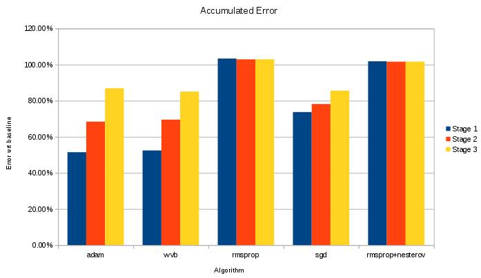
I have been testing various optimizers. The results below show how much of a signal can be recovered. To do that, we take the 1482 dimensional dataset map it through to 21 dimensions and then map it back to 1482 dimensions. After that we compare the original and recovered signal. The error we get is then compared against the most simple predictor; namely the average of the signal.
Now, the first thing we noticed is that although rmsprop style approaches go extremely fast, they do result in an average signal (literally, they just decode the signal by producing the average). Secondly, stochastic data corruption should of course not be combined with an optimizer that compensates for such noise (which the rmsprop and momentum methods do to a certain extend).
In the end, sgd turns out to retain the most ‘local patterns’, yet converges too slowly. Using adam improves the convergence speed. In this case, because mean-normalizing the data fucks up the results we actually modified adam to calculate the variance correctly.
This is of course all very beginner style stuff. Probably in a year or so I will look back at this and think: what the hell was I thinking when I did that ?
How did we come to these particular values ?
BpmDj represents each song with a 1482 dimensional vector. So I already had ~200000 entries of those and wanted to play with them. Broken down: the rhythm patterns contain 384 ticks per frequency band and we have 3 frequency bands. (thus 3*384). Aside from that we have loudness quantiles of 30 frequency bands (11*30). Which sums to about 1482 dimensions.
Then the second decission was made to stick to three layers. Mainly because google deepdream already finds high level patterns at the 3th level. No reason to go further than that I thought.
Then I aimed to reduce the same amount in each stage (/~4 as you noticed). So I ballparked the 21. And that was mainly because initially I started with an autoencoder that went 5 stages deep. It so happened I was happy at stage 21 and kept it like that so I could compare results between them.
Now, that 21 dimensional space might still be way too large. Theoretically, we can represent 2^21 classes with them if each neuron would simply say a yes/no. However, there is also a certain amount of redundancy between neurons. They sometimes find the same patterns back and so on.